
RUL estimation (Remaining Useful Life) predicts how much operational life a machine or component has left before failure, using physics-based models, data-driven machine learning, or hybrid methods, and it is what turns condition monitoring into condition-based maintenance. RUL prediction is most useful when the model family matches the available degradation data, the known failure physics, and the consequence of a wrong estimate. For safety-critical or expensive assets, the decision should also account for uncertainty, because a point estimate without a confidence range can create false precision.
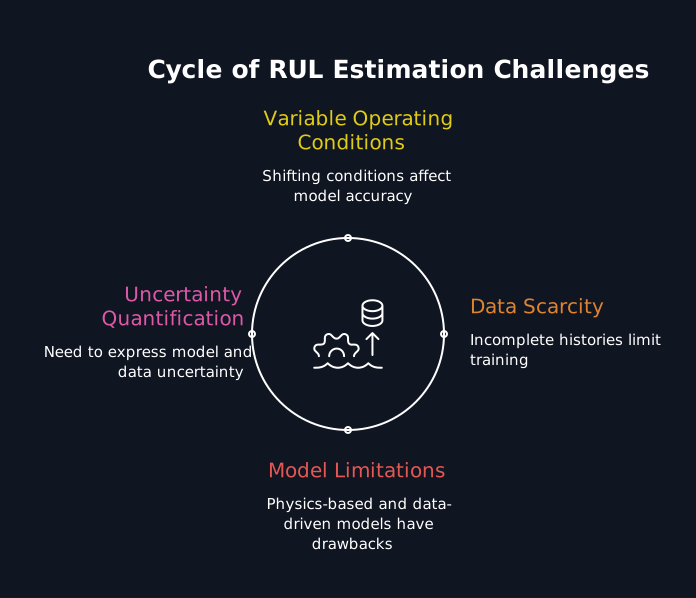
Remaining useful life estimation is harder than fault classification because the target is continuous. A classifier may answer whether a bearing is healthy or faulty. A RUL model must estimate how much useful life remains while load, speed, temperature, duty cycle, maintenance history, and failure progression can all change the relationship between today's sensor signals and the future failure point.
Variable operating conditions are one of the central problems. Research on deep domain adaptation for RUL prediction shows that models trained under one distribution can lose accuracy when operating conditions, fault modes, noise, or equipment characteristics shift in the target population. This is a form of domain shift, and it means a model validated on one machine group should not automatically be treated as reliable on another.
Data scarcity creates another constraint. Supervised RUL training is strongest when historical trajectories include the degradation process and the final failure event, but industrial fleets often have incomplete histories, censored lifetimes, replaced components, missing sensors, or only a small number of true failures. Research on transformer fleets and NASA prognostics datasets shows why lifetime data often includes incomplete or heterogeneous histories rather than clean laboratory-style sequences.
Physics-based models have a different limitation. They can encode known failure mechanisms, but their parameters may not represent the full variability of field operation. Data-driven models can adapt to complex signals, but they may be difficult to interpret and can become unreliable outside the training distribution. RUL predictions also need uncertainty quantification: Bayesian and ensemble approaches are used specifically because a single point estimate does not express model uncertainty or data uncertainty.
A degradation model estimates how quickly a component is wearing relative to a baseline or failure threshold, turning sensor observations into a usable view of system degradation. The difficulty is that degradation patterns are rarely identical across assets. Some components degrade gradually, some enter a rapid-acceleration phase near end of life, and others switch between multiple failure mechanisms.
Rapid-acceleration degradation is especially dangerous because early-life data may look stable while the final deterioration phase is much steeper. NASA-related work on turbofan RUL has explicitly separated the accelerated degradation phase because that phase can have a stronger physical relationship with remaining useful life.
Mixed-mode degradation creates another problem for early fault detection. A health indicator that tracks one mechanism well may miss another. If a bearing model is built mainly on vibration features, for example, a lubrication problem, temperature-driven mechanism, or sensor failure can create a blind spot unless the sensor set and degradation features cover those modes.
Sensor gaps can therefore become failure-mode gaps. Missing values, noisy signals, changing sensor configurations, and incomplete histories can distort the learned relationship between sensor signals and useful life. Research on RUL estimation has proposed sequence models specifically to cope with noisy and missing sensor values, which highlights that data continuity is a modeling requirement, not a data-engineering detail.
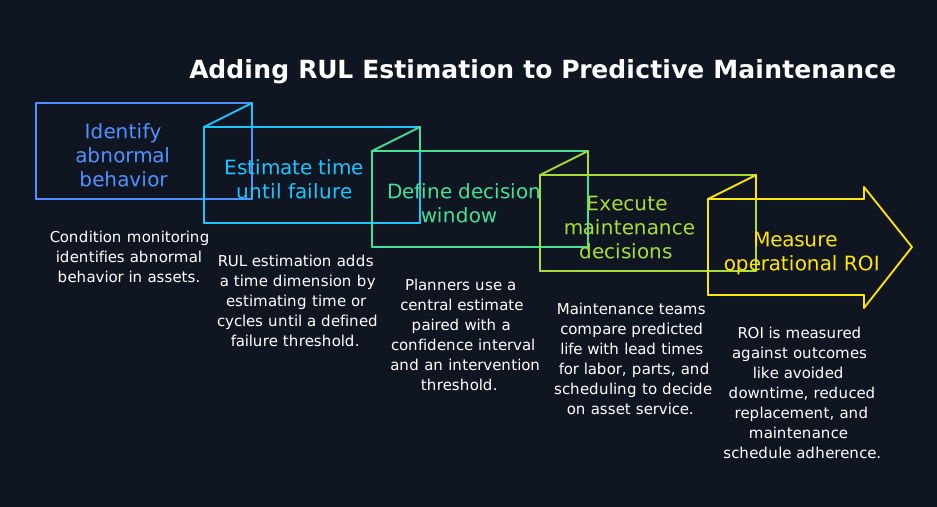
RUL tells you not just that something is degrading but when to act. Condition monitoring can identify abnormal behavior, while RUL estimation adds a time dimension that maintenance planners can use to decide whether an asset can safely remain in service, whether a spare part should be ordered, and when a maintenance window should be scheduled.
Predictive maintenance aims to perform maintenance when condition data indicates it is needed rather than relying only on fixed service intervals or waiting for a breakdown. RUL supports that goal by estimating time or cycles until a defined failure threshold, which can help convert condition monitoring into condition-based maintenance and health management. RUL estimates become more useful when paired with failure consequences, which is the logic of a risk-based maintenance approach to prioritizing assets.
For planners, the useful output is a decision window, not a single date. A practical RUL output should pair the central estimate with a confidence interval and an intervention threshold. The maintenance team can then compare the predicted life with lead times for labor, spare parts, permits, shutdown access, and production scheduling.
ROI should be measured against operational outcomes and linked back to the maintenance datasets used for validation: avoided unplanned downtime, fewer emergency interventions, reduced premature replacement, maintenance schedule adherence, and forecast accuracy against actual asset outcomes. InTechHouse's Predictive Maintenance & Industrial AI service is built around sensor integration, analytics, production deployment, and integration with maintenance systems.
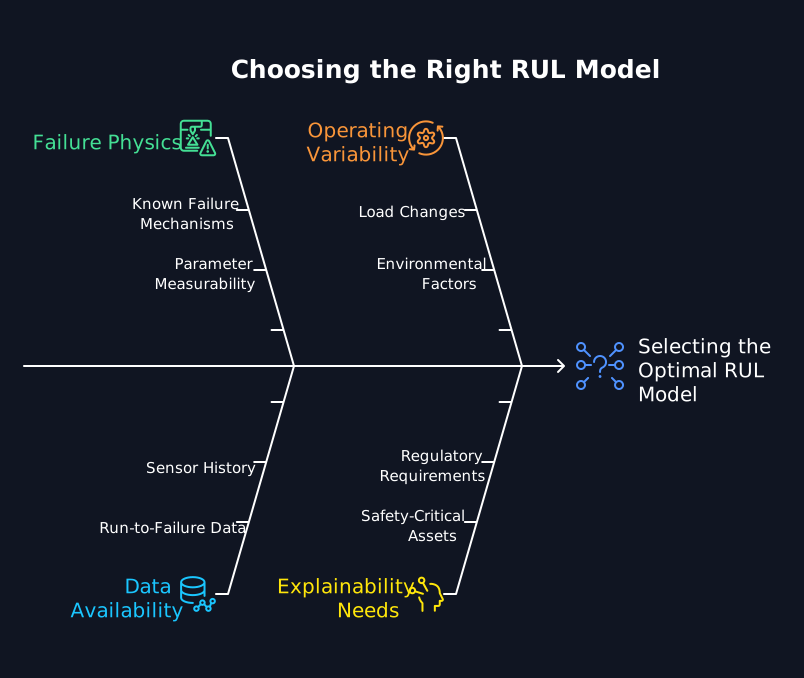
RUL prediction can be organized into physics-based, data-driven, and hybrid model families. In practical taxonomies, these are often described as physics based approaches, data driven methods, and hybrid models. Statistical lifetime and stochastic degradation models are often grouped with model-based approaches or treated as a separate analytical class, depending on the taxonomy. The right choice depends on failure physics, historical data volume, operating variability, explainability needs, and asset criticality.
Asset criticality should influence the decision. For a safety-critical asset, physical consistency, conservative uncertainty handling, and explainability may carry more weight than a small improvement in average test error. For a large fleet of similar assets with rich historical sensor data, a data-driven model can be attractive because the fleet itself provides repeated degradation examples. Hybrid models become useful when the engineering team knows part of the degradation mechanism but still needs the model to learn effects that are difficult to express analytically.
A point estimate without uncertainty creates false precision on exactly the assets where it hurts most. We build RUL models that report how sure they are, and why.
Get RUL estimates with a confidence range attached
Choose physics-based life estimation when the dominant failure mechanism is known well enough to express mathematically and the required parameters can be measured or calibrated. Fatigue crack growth is a standard example: Paris law models crack-growth rate as a function of the stress-intensity range and can be integrated toward a critical crack size to estimate remaining life.
A physics-based implementation typically needs a defined failure mechanism, equations or differential equations describing degradation, material or component parameters, load history, an observable state variable, and a failure threshold. Calibration then fits uncertain failure parameters against test or field data and updates them as new observations arrive.
Statistical and stochastic life estimation can complement this approach. Gamma-process models are used for monotonic degradation, while Weibull lifetime models are commonly used for lifetime distributions. These models are useful when the organization has population-level life data but not a complete multivariate sensor history for every asset.
Data-driven models learn the relationship between historical sensor behavior and remaining useful life.
These data driven models can use classical machine learning or deep learning, both covered in our guide to predictive maintenance with machine learning. Traditional machine learning options include Random Forests, Support Vector Regression, and Gradient Boosting; neural networks extend this approach by learning feature representations directly from sequential data. NASA RUL research has evaluated classical models, CNNs, LSTMs, and other deep architectures on C-MAPSS-style multivariate sensor data.
For supervised model training, run-to-failure trajectories are the cleanest source of labels because the failure timestamp makes RUL labels derivable at each earlier observation. Where complete trajectories do not exist, the team may need censored-lifetime methods, proxy thresholds, simulation, transfer learning, semi-supervised learning, or a hybrid model that reduces dependence on direct failure examples.
Temporal windowing matters. A single sensor snapshot may not contain enough information to distinguish stable operation from an emerging degradation trend. Windowed sequences let the model learn slope, oscillation, persistence, and cross-sensor relationships. Label engineering should also reflect the maintenance problem: the model needs a clear definition of end of useful life, not just a generic failure flag.
Model stability must be tested across operating regimes. A model that performs well on one load band can fail when applied to another if operating covariates are not represented. Domain adaptation research on RUL prediction directly addresses this problem by learning features that remain useful across changing operating conditions.
Hybrid models combine model-based degradation knowledge with data-driven learning. One pattern uses a physical model as the main degradation trajectory and trains a neural network on the residual error. Another embeds a differential equation or other physical relationship in the loss function, which is the basic idea behind physics-informed neural networks.
This is useful when the engineering team knows the broad failure mechanism but real operation introduces effects that the analytical model does not capture well. The physical component constrains the prediction, while the learnable component accounts for operating variation, hidden interactions, or imperfect parameters.
Ensemble techniques can also combine predictions produced by multiple RUL models. Stacking, boosting, or model ensembles can improve robustness when individual predictors respond differently to degradation patterns. For probabilistic maintenance planning, the training objective should also account for uncertainty rather than optimizing only a point-estimate loss.
Neural network choice should match the structure of the degradation signal rather than follow a single ranking of architectures.
CNNs, including convolutional neural networks used on multichannel time series, are useful when local patterns across channels or short temporal neighborhoods contain strong degradation information and when the model needs to learn spatial hierarchies across sensor channels. RUL research has used deep convolutional networks to learn features directly from multivariate sensor windows without manual feature engineering.
LSTMs are a common choice for sequential degradation because their recurrent structure is designed to retain temporal context. Deep neural networks built with recurrent layers can model long range dependencies when degradation unfolds over extended sequences. They are useful when the ordering and evolution of sensor readings carry more information than an isolated measurement. NASA-related studies have used LSTM-based models for engine RUL prediction and physics-informed variants.
TCNs use causal or dilated temporal convolutions to model sequence structure. They can be effective when the model needs a large temporal receptive field with parallelizable computation. Research has applied temporal convolutional models to industrial machinery and gate-valve RUL estimation.
Transformers become attractive when long-range dependencies and relationships across a long sensor history matter. Attention lets the model weight distant observations directly, and recent RUL research has evaluated Transformer variants on turbofan and bearing datasets.
Bayesian neural networks and probabilistic ensembles are appropriate when maintenance planning needs calibrated intervals around the RUL estimate. Research on Bayesian deep learning for RUL explicitly targets confidence intervals and uncertainty-aware prediction, while ensemble approaches can separate data uncertainty and model uncertainty.
Explainability should be designed into validation. Useful techniques include attention-weight inspection, feature attribution, degradation-curve visualization, sensitivity testing, and comparison against known physical variables. The goal is to provide enough evidence for engineers to understand why the estimate changed and whether the change is physically plausible.
RUL lives or dies on run-to-failure data and honest covariate labels. Data-driven methods need sensor measurements that represent degradation, while operating-condition metadata is needed to separate wear from normal changes caused by load, speed, environment, or process state. NASA C-MAPSS includes operational settings precisely because operating conditions materially affect engine signals.
Your data requirements should include:
Feature extraction should isolate indicators of wear in raw signals while preserving the degradation trend the model needs to learn. The pipeline should extract features consistently across training and current data. For industrial pipeline design, see Industrial DataOps: Best Practices for the Factory Floor.
Run-to-failure data gives the model a complete degradation trajectory with a known endpoint. NASA C-MAPSS is a standard example: its training sequences begin under normal operation, develop a fault, and continue until system failure, while test sequences stop before failure and require the algorithm to estimate the remaining cycles.
In a production dataset, record the exact failure timestamp or end-of-useful-life threshold, then segment trajectories by operating mode and asset configuration. Keep maintenance interventions visible. Replacing a component, resetting a control system, changing a lubricant, or recalibrating a sensor can break a degradation sequence and should not be hidden inside a continuous label history.
A health indicator compresses one or more sensor signals into a variable that tracks system health or degradation. It can be engineered using domain knowledge or learned by a model, but it must be monotonic enough, stable enough, or otherwise informative enough to support progression toward a failure threshold.
Failure thresholds should be defined per asset class and failure mode. A threshold might represent crack size, minimum battery capacity, maximum vibration severity, loss of efficiency, thermal limit, or another engineering boundary. If the threshold itself varies by operating condition, that uncertainty belongs in the model rather than being hidden behind one fixed number.
Condition indicators are only as good as the sensing layer that produces them, and most RUL programs inherit that layer from an existing monitoring deployment. If sensor coverage, sampling rates, or ingestion pipelines are still open questions, our guide to IoT predictive maintenance covers how that data layer gets built before any degradation model is trained.
Train and validate RUL models in a way that respects time and asset identity. Randomly mixing adjacent windows of the same trajectory across training and test data can create leakage because the model effectively sees nearly identical portions of the same degradation history on both sides of the split.
Root mean squared error is useful for overall life-estimation accuracy, but it treats early and late errors symmetrically. Prognostics benchmarks also use asymmetric scoring because overestimating useful life can be more costly or dangerous than predicting a conservative early intervention. The PHM benchmark literature explicitly uses an asymmetric score for this reason.
The model training process should include a defined loss function, temporal or asset-level cross-validation, procedures to tune hyperparameters on validation data, prediction-interval calibration, and error analysis by operating regime. Report both central accuracy and bias. A model with acceptable average squared error can still be unsafe if it systematically overestimates RUL near failure.
Statistical evaluation can also model a time-to-failure distribution rather than only a point estimate. This is useful when maintenance planning needs the probability that an asset survives past a proposed service date, not simply an expected RUL value. Bayesian and stochastic degradation methods provide a natural framework for this type of output.
A RUL model only creates value when its output becomes a scheduled work order. Production deployment therefore needs more than an inference endpoint. It needs a data path, a decision policy, ownership, and feedback after maintenance is performed.
A practical deployment can stream real time data through the industrial data platform, generate a health indicator and RUL estimate, attach uncertainty bounds, and push the result into an operator dashboard. The production service should predict RUL on each eligible asset only when data quality and model-validity checks pass. Alert logic can use both the predicted life and the confidence interval. If the lower confidence bound crosses the maintenance lead-time threshold, the system can escalate the asset for engineering review or create a CMMS work-order candidate. Wiring confidence bounds into alert logic and CMMS work orders is where many industrial AI solutions succeed or stall, since the model only pays off when maintenance planners act on it.
The CMMS integration is what closes the operational loop. InTechHouse describes predictive maintenance architectures that connect to existing OT systems and maintenance management software so predicted degradation can enter the same workflow used for planned work. Running predicted and planned jobs through one queue is a practical way to see predictive and preventive maintenance compared on real scheduling data.
Model operations also matter after launch. Input distributions, sensor quality, prediction residuals, false alarms, missed failures, and confidence calibration should be monitored continuously. For lifecycle operations, see Edge MLOps: Updating and Managing ML Models on Deployed Devices. For the sensor and data path, see Industrial IoT Architecture: Layers and Components.
RUL output only creates value once it reaches the people who schedule work, which means work orders, CMMS integration, and a defined response for every threshold. The wider program sequence around that, from asset prioritization through pilot to scale-up, is covered in our guide to step-by-step predictive maintenance implementation.
On a production line, those work orders must also fit around output targets, a tension that predictive maintenance in manufacturing has to resolve.
Benchmarking should test whether the model can estimate RUL on unseen assets, not whether it can memorize known trajectories. Public prognostics datasets provide a common reference point before an organization validates transfer to its own fleet.
NASA C-MAPSS contains multivariate run-to-failure turbofan simulations with operational settings, sensor noise, different operating conditions, and different fault-mode configurations. NASA also maintains a Prognostics Center of Excellence repository that includes PHM Challenge datasets and other RUL-relevant datasets such as milling, batteries, bearings, and electronics aging data.
Use these datasets to compare preprocessing, model training, test value, and error metrics under reproducible conditions. Then perform transfer tests across fleet subsets, operating regimes, sites, component versions, or time periods. A strong public benchmark result does not prove production readiness if the plant data follows a different distribution.
Publish the split logic, feature set, label definition, metrics, uncertainty method, and transfer-test results internally. Reproducibility makes it easier to decide whether an apparent model improvement is real or a consequence of different preprocessing.
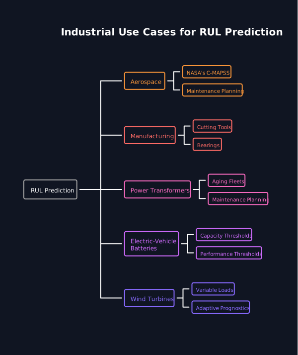
RUL prediction is useful when maintenance timing depends on degradation progression rather than a fixed calendar. The objective is to estimate RUL early enough to reduce the operational impact of asset failure. Good pilots usually target assets with observable wear signals, meaningful failure consequences, and a maintenance action that can be scheduled once the remaining useful life becomes sufficiently short.
Aerospace. NASA's C-MAPSS work is built around simulated aircraft-engine degradation and has become a major benchmark for RUL prediction. The use case is maintenance planning under changing operating conditions, where a life estimate can support decisions before a component reaches failure.
Manufacturing. RUL models have been applied to cutting tools, bearings, production machinery, and other degrading components. Manufacturing studies link RUL prediction with maintenance scheduling and avoidance of production interruptions caused by unexpected component failure.
Power transformers. Aging fleets make remaining-life planning particularly relevant. The U.S. Department of Energy reported that more than 70% of U.S. large power transformers were older than 25 years (U.S. Department of Energy, 2022), while statistical research on transformer fleets has modeled remaining-life distributions to support maintenance and capital planning.
Electric-vehicle batteries. RUL estimation supports battery health management because the endpoint can be defined by a capacity or performance threshold. Recent research evaluates data-driven and hybrid approaches using voltage, current, temperature, capacity, and cycle history to estimate useful life under changing battery conditions.
Wind turbines. RUL and prognostics are used to support maintenance decisions for assets exposed to variable loads and difficult service access. Adaptive prognostics research combines condition monitoring, damage modeling, and uncertainty quantification so model parameters can update when degradation behavior changes.
For the planned oil and gas article, use: [LINK: oil and gas predictive maintenance use cases, add after publication]. The proposed URL in the brief currently returns a not-found response.
For bearing fleets, a hybrid CNN-LSTM is a sensible pilot when vibration signals contain local spectral patterns and the degradation trajectory also depends on longer temporal behavior. CNN layers can perform feature extraction, while LSTM layers model progression over time. Bearing RUL studies have used CNN-LSTM and CNN-BiLSTM combinations for this reason.
For turbine creep-fatigue or crack-growth problems, a PINN-style model is more appropriate when the governing degradation physics can be represented explicitly. The physical loss constrains predictions while the neural component learns residual behavior not captured by the simplified model.
For battery capacity fade, physics-informed recurrent models can combine electrochemical or empirical degradation relationships with sequential learning. This is useful when the model must capture both known aging behavior and operating-history effects.
For compressor valve wear, an ensemble can be useful when multiple sensor channels or degradation indicators provide partially independent evidence. The model family should still be selected only after the failure physics and available labels are mapped. An ensemble cannot compensate for a sensor set that does not observe the target failure mechanism.
Read also:
Covariate or domain shift: Operating conditions change, but the model still assumes the training distribution. Mitigate this with operating-condition covariates, regime-specific validation, retraining triggers, and domain adaptation where appropriate.
Overfitting: A complex model learns individual training trajectories rather than general degradation features. Mitigate this with asset-level splits, regularization, early stopping, simpler baselines, and validation across sites or operating regimes.
Data scarcity: Too few failures make supervised model training unstable. Mitigate this with transfer learning, semi-supervised methods, simulation where the physics is credible, stochastic lifetime models, or hybrid architectures that encode prior engineering knowledge.
Weak labels: A maintenance replacement timestamp is treated as a true failure point even when the component still had useful life. Mitigate this by separating preventive replacement, functional failure, inspection threshold, and safety threshold events.
Poor degradation features: The model sees sensor variables that correlate with operating mode but not wear. Mitigate this with failure-mode analysis, feature stability tests, condition normalization, and engineering review of health indicators.
Uncalibrated uncertainty: The model produces a precise RUL estimate even when the current asset is unlike anything in the training set. Mitigate this with Bayesian models, ensembles, prediction-interval calibration, and explicit out-of-distribution checks.
RUL estimation should be treated as a continuously validated health management capability rather than a one-time model build. New failures, maintenance outcomes, sensor changes, and operating regimes create evidence that should feed model refinement.
Data-efficient approaches are especially relevant because true run-to-failure trajectories are expensive and often scarce. Transfer learning, semi-supervised learning, domain adaptation, physics-informed artificial intelligence, and graph-based architectures can reduce dependence on large labeled target datasets, but each still needs validation against the actual asset population.
Uncertainty quantification is another priority. Maintenance teams need to know whether an estimate is stable enough to support a scheduled intervention. Probabilistic neural networks, Bayesian methods, and ensembles provide a path toward intervals that can be calibrated against observed outcomes.
Safety implications should be monitored explicitly. In critical systems, the cost of overestimating remaining useful life may be much higher than the cost of a conservative early estimate. That asymmetry should appear in the loss function, validation metrics, escalation logic, and maintenance acceptance criteria.
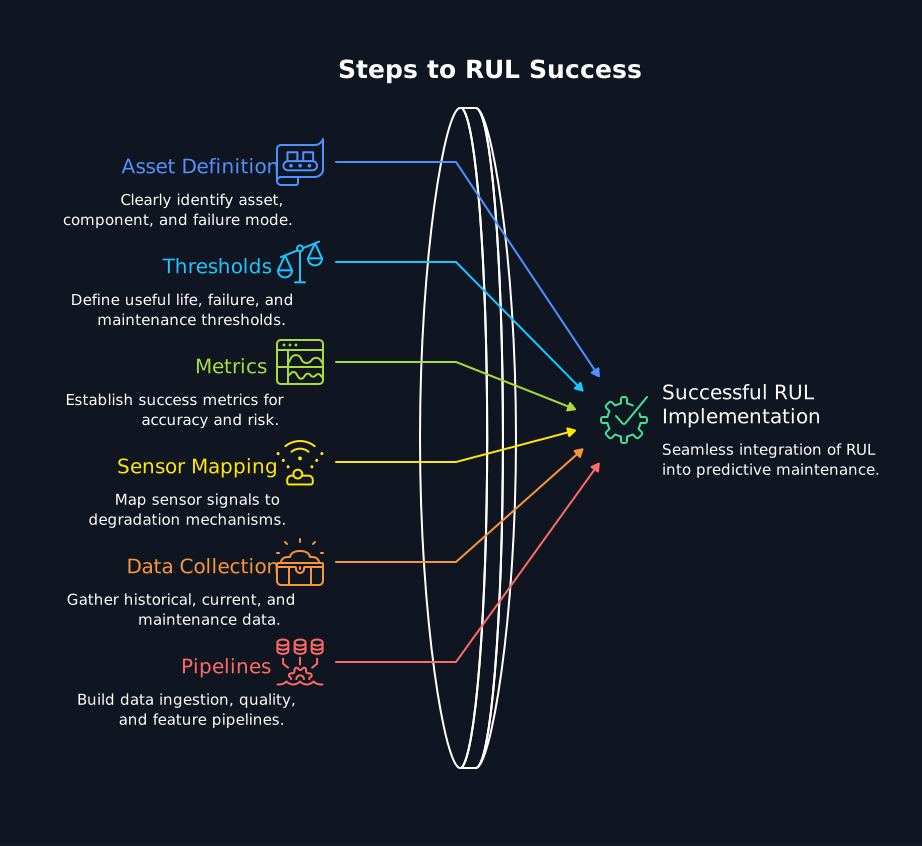
Use this checklist before moving a RUL estimation project into production:
For implementation support, see Predictive Maintenance & Industrial AI and Industrial Data Platforms & OT/IT Integration.
InTechHouse developed a predictive maintenance platform for a multinational industrial client operating subsea infrastructure, using continuous sensor data, real-time processing, anomaly detection, historical analysis, forecasting, and configurable expert logic (InTechHouse case study, accessed 2026). The published project description does not state that a dedicated RUL model, a specific neural architecture, or labeled run-to-failure trajectories were part of the delivered scope. The same architecture is directly transferable to RUL estimation by adding lifecycle labels, degradation trajectories, an appropriate physics-based, data-driven, or hybrid prediction layer, uncertainty bounds, and integration with maintenance planning. This makes the case relevant as an implementation foundation without claiming an RUL deliverable that the published evidence does not document.
Most industrial fleets have few true run-to-failure trajectories. We use hybrid physics and data-driven methods and domain adaptation to work with the history you actually have.
Work with us on censored and incomplete failure histories
Not sure where to start? We work with companies at every stage, from early ideas to enterprise-level builds. A 30-minute call can save you months of guesswork.
RUL estimation predicts how much useful operating time or how many cycles remain before an asset reaches a defined failure or intervention threshold. It gives predictive maintenance a time-to-action estimate rather than only a current condition or anomaly score.
The main methods are physics-based models, statistical or stochastic models, data-driven machine learning and deep learning, and hybrid methods that combine physical knowledge with learned behavior. The best choice depends on degradation physics, historical data, operating variability, explainability, and asset criticality.
There is no universal trajectory count that guarantees a reliable RUL model. Data needs depend on failure-mode diversity, signal dimensionality, operating regimes, label quality, model complexity, and whether the model includes a credible physics prior; the requirement should be established with learning curves and validation on held-out assets.
There is no single best neural network for every RUL prediction problem. CNNs suit local multichannel patterns, LSTMs suit sequential degradation, TCNs handle long temporal receptive fields efficiently, Transformers suit long-range dependencies, and Bayesian variants are useful when calibrated uncertainty is required.
NASA C-MAPSS and PHM Challenge datasets are widely used benchmarks for RUL algorithms, especially for turbofan-engine prognostics. NASA's Prognostics Center of Excellence repository also includes datasets for milling tools, batteries, bearings, and electronic components that support prognostics research.
Damian Ledziński, PhD Eng., is an Applied Artificial Intelligence Expert and an Assistant Professor at Bydgoszcz University of Science and Technology. He has over 15 years of academic, research, software-engineering, and technology-development experience.
His work focuses on applying artificial intelligence, machine learning, deep neural networks, and data science to complex real-world systems. His principal research and engineering interests include autonomous unmanned aerial vehicles, drone navigation and swarm intelligence, biomedical engineering, medical signal and image analysis, predictive modeling, industrial IoT, and intelligent water-management systems.
Damian has contributed to multidisciplinary R&D initiatives including AI-assisted medical diagnostics, a Polish ventilator prototype, autonomous indoor drone systems for warehouse inventory, AI-supported water-consumption analysis, virtual medical assistants, and intelligent systems combining embedded devices with machine-learning models.
He is the author or co-author of more than 30 scientific publications. His work has appeared in international scientific publications covering artificial intelligence, biomedical engineering, signal analysis, autonomous systems, environmental monitoring, and data-driven infrastructure.
Damian is a co-creator of academic programs in Engineering in Medicine, AI in Medicine, and Data Science at Bydgoszcz University of Science and Technology. He combines scientific research with hands-on implementation, translating experimental AI methods into deployable technology. He writes about applied AI, machine learning, predictive analytics, autonomous UAV systems, AI in medicine, biomedical signal processing, industrial IoT, and intelligent models in real-world systems.
Damian Ledziński's academic profiles:
https://wtie.pbs.edu.pl/pl/pracownik/damian-ledzinski
https://www.researchgate.net/profile/Damian-Ledzinski
https://scholar.google.pl/citations?user=AlQpPB0AAAAJ&hl=pl
https://ludzie.nauka.gov.pl/ln/profiles/DN6pHXU6KZm/publications/f83a8833-6060-4fae-8628-3dbf57661394
This initial conversation is focused on understanding your product, technical challenges, and constraints.
No sales pitch - just a practical discussion with experienced engineers.
Share a few details about your product and context. We’ll review the information and suggest the most appropriate next step.