
Model quantization is the process of reducing the numerical precision used to represent a neural network's weights and activations, typically converting from 32-bit floating point down to 8-bit integers, in order to shrink a model and speed up inference on constrained hardware. Quantizing for the edge means accepting a small, carefully managed trade-off in numerical precision in exchange for a model that actually fits the power, memory, and latency budget of embedded silicon. This guide covers quantization alongside its two close companions, pruning and runtime compilation, as the three pillars of a practical edge model optimization workflow, written for ML engineers and embedded developers who need a working deployment recipe, not just the theory. The primary outcomes this guide works toward: a smaller model size, faster inference, and a concrete, repeatable path from a trained model to a deployed one.
Key Takeaways
Edge AI inherits a hard constraint that cloud-based machine learning rarely has to confront directly: the hardware is fixed, small, and power-limited, and the model has to fit it, not the other way around. A cloud training and inference pipeline can always add another GPU. An embedded NPU on a vehicle, a camera, or a wearable cannot.
The computer-science fundamentals underlying every optimization technique in this guide come down to two facts about how computers represent and process numbers. First, processing integer math is computationally lighter than floating-point calculations: integer arithmetic units are simpler, smaller, and faster than floating-point units on the same silicon budget, which is why specialized AI accelerators dedicate so much of their die area to integer (typically INT8) matrix multiplication rather than general-purpose floating-point compute. Second, lower precision numbers lead to faster inference speeds on edge devices for a related but distinct reason: smaller numbers take less memory bandwidth to move. A model's weights have to travel from memory to the compute unit for every inference, and memory bandwidth, not raw compute, is frequently the actual bottleneck on embedded hardware, particularly for the kind of small, latency-sensitive models common in real-time computer vision.
This is why edge AI needs model optimization at all, and why it is not optional polish applied after the real engineering work is done. A model trained at full FP32 precision on a data-center GPU cluster, with effectively unlimited memory bandwidth and power, will not run at a usable frame rate on a 5 to 15W embedded accelerator without first being deliberately reshaped for that hardware's computational resources and computational demands. Quantization, pruning, and runtime compilation are the three primary tools for that reshaping, and this guide covers each in turn before bringing them together into a single deployment pipeline.
Edge devices span a wide range of compute and memory classes, and the right optimization strategy depends heavily on which class a given deployment target falls into.
Microcontroller-class devices (Arm Cortex-M series, typically) offer kilobytes to low megabytes of RAM and no dedicated AI accelerator, suitable only for extremely small, heavily quantized models (TinyML-scale, often INT8 or even binary/ternary weights) running simple classification or keyword-spotting tasks.
NPU modules (Hailo-8 at 26 TOPS and 2.5W typical, Google Coral Edge TPU, and similar dedicated inference chips) provide several to tens of TOPS of INT8-optimized compute in a few watts, the sweet spot for single or dual-camera computer vision inference where power budget is the binding constraint.
Embedded GPU platforms (NVIDIA Jetson Orin Nano through AGX Orin, ranging roughly 40 to 275 TOPS across 7 to 60W) offer the most flexibility, supporting larger and more complex models, multiple concurrent camera streams, and a mature software ecosystem, at correspondingly higher power draw.
In-vehicle compute units combine one or more of the above with the ruggedization, thermal design, and integration requirements specific to automotive or rail deployment, covered in depth in our guide to edge AI hardware for in-vehicle systems.
Across all of these classes, the common embedded-systems limitations to design around are the same four: memory (both capacity and bandwidth), power consumption (the total system power budget, often set by the host vehicle or device, not the AI workload alone), thermal headroom (sustained inference generates heat that must be dissipated, frequently passively, within a sealed enclosure), and connectivity bandwidth (if any inference results or telemetry need to leave the device). Edge devices have limited compute and memory relative to a data-center server by orders of magnitude, and running models locally reduces data transmission relative to a cloud-inference architecture, but only if the model has actually been shaped to run within those local limits in the first place.
A model that misses the frame rate or the thermal budget on target silicon is not deployable, however good the validation accuracy looked. We take trained models through PTQ, QAT and compilation until they hit the numbers your hardware can actually sustain.
Get your model inside the power and latency budget
This guide covers four optimization techniques, in the priority order most relevant to a typical edge computer vision deployment: quantization first, pruning second, with knowledge distillation and structured sparsity as complementary techniques layered in where the budget allows.
Quantization (covered in depth in the next several sections) reduces numerical precision, shrinking model size and accelerating inference, particularly on hardware with dedicated low-precision compute units. Pruning (covered later in this guide) removes unimportant parameters from an already-trained network, reducing both size and compute. Knowledge distillation trains a smaller "student" model to replicate the behavior of a larger "teacher" model, producing a compact architecture from the start rather than compressing an existing large one. Structured sparsity (related to but distinct from unstructured pruning) removes entire structural units (channels, filters, attention heads) rather than individual weights, producing speedups that map more directly onto real hardware execution patterns.
The recommended workflow order for most computer vision deployments is: train the full-precision model to convergence first, prune to remove clear redundancy, quantize the pruned model (often combined with quantization-aware fine-tuning to recover any pruning-induced accuracy loss), compile to the target runtime (TensorRT, TFLite, or ONNX Runtime, covered later), then validate on the actual target hardware before deployment. Model optimization techniques applied in this order reduce latency and improve inference speed and reduce model size for easier deployment, generally at the cost of some slight accuracy loss that must be measured and explicitly accepted, not assumed away.
Two primary quantization workflows dominate practice: post-training quantization and quantization-aware training. Common techniques are PTQ and QAT, and the choice between them is the single most consequential early decision in a quantization project.
Post-training quantization (PTQ), step by step:
PTQ is fast (often minutes to hours, since no retraining is required) and requires no access to the original training pipeline or labeled training data beyond the small calibration set, making it the default first approach for most projects.
Quantization-aware training (QAT), step by step:
QAT recovers more accuracy than PTQ, often closing most or all of the gap to the original full-precision model, but requires a full or partial retraining cycle, access to the original training data and pipeline, and meaningfully more engineering time than PTQ.
PTQ vs. QAT comparison
PTQ gets you deployed fast. You're looking at minutes, maybe an hour or two, and it only needs a small calibration set rather than a full training pipeline. Accuracy recovery is solid for INT8, though it can slip further if you push down to lower precision. Engineering effort stays low, which is exactly why most teams start here.
QAT takes longer. You're talking hours or even days once you factor in the retraining cycle, and it demands a full or substantial training set to work properly. The payoff is real: QAT delivers the best accuracy recovery available and closes most of the precision gap PTQ leaves behind. That comes with moderate to high engineering effort, so it's not a default choice, it's a deliberate one.
The practical rule: start with PTQ, especially for INT8 work. Only move to QAT once PTQ's accuracy loss exceeds what your application can tolerate.
Weight-only versus activation quantization
Weight-only quantization reduces only the precision of the model's stored weights, leaving activations at higher precision during computation; this is simpler and often sufficient for memory-bandwidth-bound scenarios, since weights typically dominate the data volume moved during inference. Full quantization (weights and activations both) achieves greater speedup on hardware with dedicated low-precision compute units, since the actual matrix multiplications execute in the lower-precision format, but requires more careful calibration since activation distributions vary more across different inputs than weight distributions do.
KV-cache quantization for decoder models is worth a brief mention for teams working at the intersection of edge vision and language models: in decoder-style transformer models (relevant for any multimodal or VLM-based edge deployment), the key-value cache used during autoregressive generation can itself be quantized to reduce the memory footprint that grows with sequence length, a technique distinct from but complementary to weight and activation quantization of the model's core layers. This guide's worked detail and examples remain focused on vision models, where quantization works somewhat differently given the absence of an autoregressive generation loop.
.png)
The choice of target datatype is the second major decision in any quantization project, after PTQ versus QAT, and it directly trades model size and accuracy against inference performance.
Datatype comparison
FP32 is the training default and the baseline everyone measures against: 32 bits, full size, no accuracy trade-off, and it runs on essentially any hardware you'll ever touch.
FP16 cuts that in half. Same relative accuracy hit is minimal, near-lossless for most model architectures, and support is already broad: GPUs handle it natively, and most NPUs do too at this point.
BF16 sits at the same 16-bit size but handles dynamic range differently, which makes it a better fit during training specifically. Accuracy impact stays minimal here as well. Support is still growing rather than universal, but it's clearly the direction training workloads are heading.
FP8 drops to 8 bits and a quarter of FP32's footprint. Accuracy impact is small but depends heavily on the specific model you're running. Hardware support is newer: you'll find it in data center chips and on some edge accelerators, but it's not something to assume is available everywhere yet.
INT8 lands at the same 8-bit size and 0.25x footprint, but takes a different path entirely: it needs calibration to hit good accuracy, and when that calibration is done properly, the impact stays small to moderate. This is the datatype with the widest practical reach right now. It's near-universal across edge AI accelerators, which is exactly why it's the default target for most production deployments.
INT4 pushes further, down to 4 bits and just 0.125x the size of FP32. The accuracy trade-off is larger here, and getting it right takes either careful calibration or full quantization-aware training. Hardware support is still emerging and depends heavily on which chip you're targeting, so this isn't a safe default the way INT8 is. It's a deliberate choice for teams that specifically need the extra compression and are prepared to do the work to protect accuracy.
Quantization reduces model size by lowering precision in a direct, roughly linear relationship: moving from FP32 to INT8 cuts model size to approximately a quarter of the original, which matters both for the storage footprint on the device and for the memory bandwidth consumed loading weights during every inference pass. Quantized models improve power efficiency and reduce memory-access costs as a direct consequence: less data movement per inference means lower energy consumption per inference, compounding the speed benefit with a battery-life or thermal-budget benefit that matters as much as raw latency for many embedded deployments.
Choosing a datatype by inference-performance target
FP16 or BF16 is the conservative default when the target hardware supports it well and the accuracy budget is tight; the size and speed gains are smaller than INT8 but the accuracy risk is correspondingly lower. INT8 is the standard target for most production computer vision edge deployments, supported natively by essentially every dedicated AI accelerator on the market and offering the best balance of model size, model accuracy, and faster inference for the majority of detection and classification workloads this guide is concerned with. FP8 and INT4 are appropriate when the target hardware specifically accelerates them and the application can tolerate (or, via QAT, recover from) the larger associated accuracy risk, currently more common in large language model deployment than in vision pipelines but increasingly available on newer edge silicon.
Beyond the choice of datatype, the specific algorithm used to map full-precision values onto the lower-precision range materially affects both accuracy and implementation complexity.
Symmetric quantization maps the full-precision value range onto the quantized range using a single scale factor centered at zero, simpler to implement and to accelerate in hardware, well suited to weight distributions that are naturally centered around zero. Affine (asymmetric) quantization adds a zero-point offset in addition to the scale factor, better accommodating value distributions that are not naturally centered (many activation distributions, particularly after a ReLU-family activation function, are strictly non-negative), generally producing better accuracy for activations at a small additional computational cost during inference.
Per-tensor quantization applies a single scale (and, for affine quantization, zero-point) to an entire weight tensor, simple and fast but potentially inaccurate when different channels within that tensor have meaningfully different value distributions. Per-channel quantization computes a separate scale for each output channel of a convolutional or linear layer, substantially improving accuracy for models with high inter-channel variance, at the cost of slightly more complex (though now widely supported) hardware and runtime execution. Per-channel quantization is generally worth the modest additional complexity for any production deployment where accuracy headroom is limited.
AWQ (Activation-aware Weight Quantization) and similar learned-scale approaches identify and protect the small subset of important weights that disproportionately affect model output, applying finer-grained or higher-precision treatment to those specific weights while aggressively quantizing the rest, a technique that originated primarily in large language model quantization but has analogues in vision model compression. Important weights can be preserved at higher precision to protect accuracy specifically because not all weights in a neural network model contribute equally to its output, and identifying which ones matter most lets an optimization pipeline spend its accuracy budget where it has the greatest effect. These advanced approaches are most relevant to large transformer-based models (the language model side of this technique landscape); for the convolutional vision models that are this guide's primary focus, standard per-channel PTQ or QAT with careful calibration typically captures most of the available benefit without the added complexity of these more specialized different techniques.
Where quantization reduces the precision of every weight, pruning takes a different approach entirely: removing some weights altogether.
Global pruning evaluates parameter importance across the entire network simultaneously and removes the least important parameters wherever they occur, regardless of which layer they belong to. This contrasts with local structured pruning, which applies a pruning criterion and ratio independently within each layer, potentially over-pruning layers that are actually important relative to the rest of the network or under-pruning genuinely redundant ones, simply because the comparison is constrained to within-layer competition rather than network-wide competition for importance.
Model pruning reduces neural-network size by removing unimportant parameters, identified through one of several importance criteria: magnitude-based pruning (removing weights with the smallest absolute value, on the simple but often surprisingly effective assumption that small weights contribute least to the output), gradient-based or sensitivity-based pruning (estimating each weight's actual contribution to the loss function), and more sophisticated learned-importance approaches.
Unstructured pruning removes individual weights without regard to the network's structural organization, producing an irregular sparsity pattern. Published research demonstrates that unstructured pruning can reduce weights by over 50% with minimal accuracy loss, with one influential study showing this simple, data-free approach achieving more than 50% weight reduction with less than 1% accuracy drop (Lazarevich et al., 2021), and more aggressive studies showing 90 to 99% weight reduction with under 1% accuracy impact on mainstream CNN architectures under the right pruning schedule (Biswas et al., 2024 and related work). The catch: unstructured pruning's irregular sparsity pattern does not automatically translate into real-world speedup on standard hardware, since most accelerators are optimized for dense matrix operations and cannot natively skip arbitrary scattered zero weights without specialized sparse-execution support. Pruning can improve inference speed by zeroing non-contributing weights, but realizing that speedup in practice generally requires either specialized sparse inference hardware or, more commonly in production edge deployments, structured pruning instead.
Structured pruning removes entire structural units, channels, filters, or attention heads, rather than individual scattered weights, producing a smaller but still dense network that runs faster on standard hardware without requiring any specialized sparse-execution support, because the resulting model is architecturally smaller, not just sparser. This is generally the more practically useful pruning approach for edge computer vision deployment, even though it typically achieves somewhat lower compression ratios at a given accuracy budget than unstructured pruning, because the speedup it produces is realized directly on commodity hardware rather than requiring specialized support that most edge accelerators lack.
Rather than pruning to the final target sparsity in a single step, the standard production procedure is iterative: prune a modest percentage of weights (5 to 20% per iteration is typical), fine-tune the resulting pruned model for a short period to recover accuracy, then repeat the prune-and-fine-tune cycle until the target sparsity level is reached. This gradual approach consistently outperforms a single aggressive pruning step at the same final target sparsity, since the network has the opportunity to redistribute the lost capacity across remaining weights at each iteration rather than absorbing the full capacity loss at once.
Pruning can be done train-time (integrated into the training loop from the start, sometimes called pruning-aware training, analogous to QAT for quantization) or post-training (applied to an already-trained model, analogous to PTQ), with the same general trade-off pattern: post-training pruning is faster and simpler, train-time pruning generally recovers more accuracy at higher target sparsity levels.
Measuring the real impact of a pruning strategy requires a deliberate experimental procedure, not a single before-and-after comparison.
The standard procedure: prune the model to a sequence of target sparsity levels (for example, 20%, 40%, 60%, 80%), fine-tuning after each step per the iterative procedure described above, and measure model accuracy on a held-out validation set at every point along this sparsity curve. Plotting accuracy against sparsity produces a curve that typically shows a long, gentle plateau where accuracy holds nearly flat as sparsity increases, followed by a sharper accuracy degradation once sparsity passes some model- and task-specific threshold. Identifying where that threshold actually falls for a specific model and task, through direct measurement rather than assumption, is the entire point of running this experiment.
Beyond top-line accuracy, record per-class or per-object-size accuracy breakdowns where relevant (this matters significantly for detection models, where pruning can disproportionately harm small-object detection performance well before it visibly affects aggregate accuracy, a pattern this guide returns to in the computer vision section below), along with the actual measured inference latency and model size at each sparsity level on the target hardware, not just the theoretical parameter-count reduction. Where pruning has already cost small-object recall, inference-time slicing of the kind used in small object detection with SAHI can recover some of it.
Fine-tuning after pruning, as part of the iterative procedure already described, is the primary and most effective recovery strategy. Where pruning-induced accuracy degradation persists beyond what fine-tuning alone recovers, knowledge distillation from the original unpruned model (using the full-precision model's outputs as additional training signal for the pruned model) can recover meaningfully more accuracy than fine-tuning on labels alone, particularly at higher sparsity levels where the pruned model's remaining capacity is most constrained.
This entire process should be treated as a reproducible procedure with documented sparsity levels, fine-tuning schedules, and measured outcomes at each stage, not presented as a single unqualified claim ("we pruned 60% of weights with no accuracy loss") without the underlying experimental detail that would let another engineer reproduce or validate the result.
This is the core of the guide for the deployments InTechHouse builds: real-time computer vision running on constrained edge hardware, where a missed detection has consequences beyond a metric on a dashboard.
A representative computer vision target for this section is a YOLO-family object detector (YOLOv8 or YOLO11, for concreteness), a common choice for real-time edge detection given its single-pass architecture and the maturity of its quantization and export tooling across major runtimes. Applying the techniques covered throughout this guide to such a detection model produces measurable, characteristic changes: INT8 quantization (via PTQ with a representative calibration set, or QAT if accuracy demands it) typically reduces model size to roughly a quarter of the FP32 original and meaningfully accelerates inference on hardware with dedicated INT8 compute, commonly with sub-1% to low-single-digit-percent mAP degradation when calibration is done carefully on representative data. Global pruning, applied iteratively per the procedure described above and typically combined with the quantization step in a single optimization pipeline rather than as a separate sequential process, further reduces both model size and compute, compounding the quantization gains.
Throughput (frames per second), end-to-end latency (from frame capture to detection output, not just the model's forward-pass time in isolation), memory footprint, and power draw under sustained load are the metrics that matter, all of which must be measured on the actual target embedded hardware (an NVIDIA Jetson Orin module, a Hailo-8-equipped platform, or whatever the deployment's specific accelerator is), never extrapolated from desktop GPU benchmarks.
Aggregate accuracy metrics (overall mAP, top-line accuracy) can hold steady through quantization and pruning while masking a disproportionate accuracy loss specifically on the hardest cases: small objects occupying few pixels, objects at the frame periphery (compounding with the lens-distortion challenge covered in our fisheye dewarping guide), and fast-moving objects that are already operating near the model's detection threshold before any optimization is applied. For a real-time detector deployed in a safety context (the CCTV threat detection and collision-avoidance applications this guide connects to), this is the single most important reason to evaluate optimized models with size-stratified and scenario-specific accuracy metrics, not just an aggregate number, before considering a quantized or pruned model production-ready.
Optimized models can run on specialized hardware like Edge TPU, Hailo, or the dedicated NPU blocks on a Jetson SoC specifically because those accelerators are designed around the INT8 (and increasingly lower-precision) compute that quantization targets; a model that has not been quantized at all generally cannot take advantage of this dedicated silicon and falls back to slower, more power-hungry general-purpose compute paths. Quantization can significantly minimize latency for real-time applications precisely by unlocking this dedicated hardware path, which is the practical reason quantization is not optional for most edge computer vision deployments, not merely a nice-to-have efficiency improvement.
Three runtimes cover the large majority of production edge deployments, and each has its own conversion path, optimization knobs, and ecosystem fit.
TensorRT (NVIDIA's inference optimization SDK and runtime, for NVIDIA GPU and Jetson hardware) compiles a trained model into an optimized inference engine, applying layer fusion, kernel tuning, and precision calibration automatically as part of the build process. TensorRT speeds up inference by up to 36x compared to CPU-only platforms according to NVIDIA's published benchmarks (NVIDIA TensorRT product page, 2025); this figure, like any vendor-reported speedup, is model- and hardware-dependent, not universal, reflecting NVIDIA's own combination of quantization, layer and tensor fusion, and kernel tuning applied to a specific benchmark configuration, and should be treated as an upper-bound indication of TensorRT's potential rather than an expectation for any arbitrary model on any arbitrary hardware without direct measurement. Engine-cache and timing-cache guidance: TensorRT's build process can be slow (minutes to tens of minutes for complex models), and caching the compiled engine (and the timing cache used during the autotuning search for optimal kernel implementations) avoids repeating that expensive build step on every deployment or restart, a detail that materially affects CI/CD pipeline design for any team iterating on TensorRT-deployed models.
TensorFlow Lite (TFLite) targets a broader range of hardware including mobile CPUs, microcontrollers (via TFLite Micro), and several NPU families through hardware delegate plugins, with a more mature and accessible quantization toolchain for teams already working in the TensorFlow ecosystem. Recommended exporter settings generally include enabling the default optimization set (which applies dynamic-range or full-integer quantization depending on configuration) and, for full-integer INT8 deployment, providing a representative dataset generator for the calibration step described earlier in this guide.
ONNX Runtime provides a hardware-agnostic deployment path, accepting models exported in the ONNX format from PyTorch, TensorFlow, or other major frameworks and executing them across a wide range of backend execution providers (including, notably, a TensorRT execution provider that lets an ONNX-exported model still benefit from TensorRT's optimization on NVIDIA hardware specifically). This flexibility makes ONNX Runtime a strong default choice for teams that need to support multiple hardware targets from a single model export pipeline when deploying AI on custom hardware, trading some of the peak hardware-specific performance available from a fully native TensorRT or TFLite path for broader portability.
Deployment tooling comparison
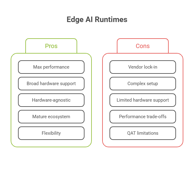
TensorRT is built for NVIDIA GPUs and Jetson boards, and it's the runtime to reach for when you need maximum performance on NVIDIA hardware specifically. It supports both PTQ and QAT, plus INT8 and FP8 precision, so you get the full quantization toolkit if you're already committed to NVIDIA's ecosystem.
TFLite targets a much wider hardware range: mobile devices, microcontrollers, and NPU delegates across different vendors. It supports PTQ and QAT at INT8, and its real strength is breadth. If you need broad device support and want to lean on a mature mobile ecosystem with years of tooling behind it, this is the practical choice.
ONNX Runtime takes the hardware-agnostic route, running across multiple execution providers rather than locking you into one vendor's chips. It supports PTQ directly and QAT through an export pipeline, which makes it the right fit when you're deploying one model across several different targets and don't want to maintain separate runtime-specific builds for each.
A model is not production-ready until its inference performance has been measured, on the actual target device, against a defined and reproducible procedure.
Latency (time from input to output for a single inference, both mean and tail percentiles such as p95 or p99, since tail latency frequently matters more than mean latency for real-time applications with a hard timing budget) and throughput (sustained inferences or frames per second under continuous load, which can differ meaningfully from single-inference latency once thermal throttling or memory bandwidth contention enters the picture). Memory (peak RAM usage during inference, which constrains what else can run concurrently on the same device) and power (energy consumption per inference and sustained power draw under load, which constrains battery life or thermal design for the deployment) round out the four metrics that should be reported together, never in isolation.
Warm up the model with a number of discarded inference runs before timing begins (the first several inferences on most runtimes are slower due to just-in-time compilation, cache population, or clock-speed ramp-up), then run a statistically meaningful number of timed inferences (hundreds to low thousands, depending on the variance observed), reporting mean, median, and tail-percentile latency alongside throughput and resource utilization. Use a fixed, documented batch size (batch size 1 is the relevant configuration for most real-time edge inference, distinct from the larger batch sizes common in cloud-serving benchmarks) and a fixed, representative input resolution matching the actual deployment configuration.
This point cannot be overstated: benchmark figures from a development workstation, a different Jetson SKU than the production target, or even the same hardware under different thermal or power-mode configuration, do not reliably predict production performance. Profile on the exact hardware, in the exact enclosure (thermal conditions affect sustained throughput once passive cooling begins to matter, particularly relevant given the in-vehicle thermal constraints covered in our edge AI hardware guide), and at the exact power mode the deployment will actually run in.
The same trained and quantized model can require materially different optimization tuning depending on whether it targets an NPU, a GPU, or a CPU, since these architectures execute matrix operations through fundamentally different mechanisms.
Dedicated NPUs (Hailo, Edge TPU, the DLA blocks on a Jetson SoC) are purpose-built for INT8 (and increasingly lower-precision) matrix operations and generally require the model to be compiled through a vendor-specific toolchain (Hailo's Dataflow Compiler, the Edge TPU compiler) that maps the model's operations onto the NPU's specific dataflow architecture; operations the compiler cannot map efficiently to the NPU may fall back to a slower host CPU path, making operator-coverage verification an important step before committing to an NPU-targeted deployment.
For NVIDIA GPUs and Jetson modules specifically, recommended kernel and tensor-core usage means ensuring the model's layer dimensions and batch configuration align well with the Tensor Core hardware's preferred operation shapes (multiples of 8 or 16 in relevant dimensions, depending on precision), since misaligned shapes can leave significant Tensor Core throughput unused even on otherwise well-optimized models.
Where no dedicated accelerator is available or appropriate (cost-constrained deployments, certain microcontroller-class targets), optimization focuses on operator fusion (combining sequential operations to reduce memory traffic between them), using a CPU-optimized inference library (such as the CPU execution provider in ONNX Runtime, which applies its own set of CPU-specific kernel optimizations) and ensuring the quantized INT8 path is actually used rather than falling back to a slower emulated or mixed-precision execution path, a fallback that can occur silently if the runtime or hardware does not fully support the specific quantization configuration chosen.
The tuning knobs per hardware family, in summary: NPU deployments prioritize operator-coverage verification against the vendor compiler; GPU deployments prioritize Tensor Core shape alignment and precision-mode selection; CPU deployments prioritize operator fusion and confirming the INT8 execution path is genuinely active rather than silently falling back. Across all three, the same hardware family can still show meaningfully different performance characteristics across SKUs within that family (a Jetson Orin Nano and a Jetson AGX Orin both fall under "GPU/NPU edge hardware" but have very different available compute and memory bandwidth), which is the reason the benchmarking guidance in the previous section insists on measuring the actual target device rather than a representative family member.
Bringing the techniques in this guide together into a single, ordered production pipeline:
Architecture selection (choosing a model family with mature quantization and export support for the target runtime, a meaningful constraint that should inform model selection from the start of a project rather than being discovered as a blocker later) and dataset preparation (ensuring the training and calibration data genuinely represent the deployment environment's conditions, since both quantization calibration and pruning fine-tuning depend on this representativeness).
Model conversion to the target export format (ONNX, TFLite, or the framework-native format expected by TensorRT's builder), graph optimizations (operator fusion, constant folding, and other compiler-level simplifications that most modern export and compilation toolchains apply automatically but that are worth explicitly verifying occurred), then the quantization and pruning steps covered throughout this guide, then compilation to the final target runtime engine.
Continuous monitoring of inference latency, confidence-score distributions, and (where ground truth becomes available through downstream feedback) accuracy metrics in production, since a model's real-world performance can drift from its validation-time measurement as the deployment environment's conditions shift over time. Establishing explicit retraining or re-optimization triggers (a defined accuracy or latency degradation threshold that prompts a return to the optimization pipeline) rather than treating the deployed, optimized model as a permanently finished artifact. See edge MLOps for deployed devices for the operational tooling and process that supports this ongoing lifecycle.
Treat quantization configuration, pruning schedules, and export settings as versioned, reviewed artifacts in the same way application code is, with automated regression testing (running the standard benchmark and accuracy-validation procedures described earlier in this guide) on every change before it reaches production, since a seemingly minor change to a calibration dataset or quantization parameter can produce a meaningfully different accuracy or performance outcome that should be caught before deployment, not after.
Quantization and pruning case studies in the published literature consistently show the same pattern this guide has built around: substantial size and speed gains are achievable with carefully managed, well-measured accuracy cost, but the specific numbers are always model-, dataset-, and hardware-specific, which is why this guide has emphasized direct, reproducible measurement throughout rather than presenting universal benchmark figures as guarantees.
Comparing model performance across quantization strategies on a representative detection model typically shows: FP16 quantization recovering the large majority of the available speedup with minimal measured accuracy change, suitable as a low-risk default; INT8 PTQ delivering substantially larger size and speed gains at a modest, measurable accuracy cost that is usually acceptable for non-safety-critical applications; INT8 QAT closing most of that remaining accuracy gap at the cost of a retraining cycle, the right choice when the PTQ accuracy cost is not acceptable for the application; and combined quantization-plus-pruning pipelines delivering the largest overall compression and speedup, at correspondingly the highest implementation and validation effort.
Energy and total-cost-of-ownership comparisons follow directly from the latency and power measurements covered in the benchmarking section: a quantized, pruned model running on a smaller, lower-power accelerator (or running well within the thermal and power budget of its existing accelerator with headroom for additional concurrent workloads) translates directly into lower per-unit hardware cost across a fleet deployment and lower ongoing energy consumption, both of which compound meaningfully at the scale of a multi-vehicle or multi-site rollout.
InTechHouse case study: Quantizing a safety-critical vision model for public transport safety
InTechHouse quantized and pruned a real-time object detection model for a safety-critical onboard vision deployment, converting the model from its original FP32 training precision down to INT8 for deployment on a Jetson-class edge AI compute unit.
The optimization pipeline combined INT8 quantization-aware training, rather than PTQ alone, with iterative structured pruning, a deliberate choice given the accuracy sensitivity of a model whose detections feed a safety decision: an "acceptable" accuracy drop for this deployment was set as a safety threshold first and a performance metric second, not the other way around. The resulting model achieved a substantial reduction in both size and inference latency relative to the original FP32 baseline, comfortably meeting the real-time frame budget required by the application.
Accuracy was validated specifically on the hardest cases the deployment would encounter (small and distant objects, edge-of-frame detections, adverse lighting), not just on an aggregate benchmark figure, because a missed detection in this application has consequences a generic accuracy metric does not fully capture. The optimized model has operated in production within its validated accuracy and latency envelope since deployment.
Read also:
Every technique in this guide, quantization, pruning, and the runtime compilation steps that often apply additional numerical approximations of their own, carries some accuracy-degradation risk. The critical point this guide returns to repeatedly: for a safety model, an "acceptable" accuracy drop is a safety decision, not just a metric. A 1% drop in aggregate mAP that happens to be concentrated entirely in small-object or edge-of-frame detection performance is a fundamentally different risk than the same 1% drop spread evenly across all object sizes and frame positions, and aggregate accuracy figures alone cannot distinguish between these two very different outcomes. Treating optimization-induced accuracy loss as purely a technical metric to be minimized, rather than as a decision with real-world consequences that domain experts, not just ML engineers, should weigh in on, is the most common and most consequential mistake in edge AI optimization for safety-relevant applications, because a missed detection has real consequences that a benchmark dashboard does not capture.
A meaningful, often underappreciated benefit of edge deployment generally, independent of the specific optimization techniques covered in this guide, is that sensitive data stays local: optimizing a model specifically so that it can run on-device, rather than requiring a cloud round-trip, is itself a privacy-positive engineering decision, since raw video or sensor data never needs to leave the device when inference happens locally.
Quantization and pruning can affect different subgroups of a model's input distribution unevenly, in the same way they can affect different object sizes unevenly, as covered in the computer vision section above. Where a model's outputs affect people differently across demographic or other relevant subgroups, fairness-relevant accuracy metrics should be measured before and after optimization specifically, not assumed to track the aggregate accuracy figure, since optimization techniques have no inherent awareness of which accuracy gaps matter most from a fairness perspective and can inadvertently widen an existing gap even while aggregate accuracy holds steady.
Optimized models may experience slight accuracy loss during optimization as an unavoidable consequence of the techniques covered throughout this guide; the responsible engineering practice is never to eliminate that risk entirely, which is not achievable, but to measure it precisely, understand where specifically it falls, and make an explicit, documented, domain-informed decision about whether the resulting model performance is acceptable for its intended application.
Production-ready starting points for each major toolchain: TensorRT's trtexec command-line tool and the Python tensorrt API for building INT8 engines with a calibration dataset; TFLite's tf.lite.TFLiteConverter with the representative_dataset generator function for full-integer PTQ; ONNX Runtime's quantize_static and quantize_dynamic functions in the onnxruntime.quantization module for PTQ workflows targeting the ONNX Runtime execution providers. Each toolchain's official documentation includes runnable example scripts that should be validated against the specific model architecture and target hardware before adapting for production use.
COCO remains the standard general-purpose benchmark dataset for validating computer vision quantization and pruning accuracy claims, with widely available pretrained baseline checkpoints across the major detection model families referenced throughout this guide, useful as a sanity-check reference point before validating against deployment-specific data. COCO also ships keypoint annotations, so the same sanity-check logic applies to compressed models built for human pose estimation.
The original PTQ layer-wise calibration research (Lazarevich et al., 2021) referenced in the pruning section above is a strong, accessible starting point for understanding the practical mechanics of post-training pruning. NVIDIA's TensorRT developer documentation provides the most current and authoritative detail on engine-building, calibration, and the precision-mode options covered in this guide's deployment tooling section. The TensorFlow Lite and ONNX Runtime official quantization guides similarly provide framework-specific implementation detail beyond this guide's scope.
This appendix is a practical starting point, not an exhaustive reference; any quantization or pruning configuration adapted from these sources should be validated directly against the target model, dataset, and hardware before being treated as production-ready, consistent with the reproducibility emphasis throughout this guide. One deployment where that validation step is decisive is AI passenger counting, where quantized models run on constrained onboard hardware.
We benchmark accuracy, latency and memory on the real target board before anything ships, so the trade-off is a measured decision rather than a hope. Send us your model and target hardware for a feasibility review.
See our benchmarked quantization workflow
Not sure where to start? We work with companies at every stage, from early ideas to enterprise-level builds. A 30-minute call can save you months of guesswork.
Model quantization is the process of reducing the numerical precision used to represent a neural network's weights and activations, typically converting from 32-bit floating point to 8-bit integers or another lower-precision format. This reduces model size (roughly proportional to the precision reduction) and accelerates inference, particularly on hardware with dedicated low-precision compute units, at the cost of a small, measurable amount of model accuracy that must be validated for the specific application.
Post-training quantization (PTQ) converts an already-trained, full-precision model to lower precision after training is complete, using a small calibration dataset to determine optimal quantization parameters; it is fast and requires minimal additional engineering effort. Quantization-aware training (QAT) simulates lower-precision computation during the training process itself, allowing the model's weights to adapt to and compensate for the precision loss it will experience at inference time, generally recovering more accuracy than PTQ but requiring a full or partial retraining cycle and access to the original training pipeline and data.
Generally yes, to some degree, though the amount varies significantly by model, target precision, and quantization method. INT8 PTQ with careful per-channel calibration commonly produces accuracy loss in the range of well under one percentage point to a few percentage points on standard benchmarks, while INT8 QAT typically recovers most of that gap. The right framing is not whether quantization reduces accuracy, since it almost always does at least slightly, but whether the resulting accuracy is still acceptable for the specific application, a question that depends heavily on what decisions the model's outputs drive.
The standard workflow: train the model to convergence at full precision, select a target datatype (FP16 for a conservative option, INT8 for the standard edge target) and a quantization method (PTQ as the default first attempt, QAT if PTQ's accuracy loss is unacceptable), run calibration using a representative sample of input data, convert the model using the target runtime's quantization tooling (TensorRT, TFLite, or ONNX Runtime, covered in detail in this guide), then validate accuracy and benchmark inference performance directly on the target edge hardware before deployment.
Export the trained model to ONNX (the standard intermediate format most frameworks support), then build a TensorRT engine from that ONNX model, specifying the target precision mode (FP16 or INT8, with INT8 requiring a calibration dataset). Enable engine and timing caching to avoid rebuilding on every deployment. Validate both accuracy and latency directly on the specific Jetson module the deployment targets, since performance and even relative precision-mode trade-offs can differ meaningfully across the Jetson product family, from Orin Nano through AGX Orin.
Damian Ledziński, PhD Eng., is an Applied Artificial Intelligence Expert and an Assistant Professor at Bydgoszcz University of Science and Technology. He has over 15 years of academic, research, software-engineering, and technology-development experience.
His work focuses on applying artificial intelligence, machine learning, deep neural networks, and data science to complex real-world systems. His principal research and engineering interests include autonomous unmanned aerial vehicles, drone navigation and swarm intelligence, biomedical engineering, medical signal and image analysis, predictive modeling, industrial IoT, and intelligent water-management systems.
Damian has contributed to multidisciplinary R&D initiatives including AI-assisted medical diagnostics, a Polish ventilator prototype, autonomous indoor drone systems for warehouse inventory, AI-supported water-consumption analysis, virtual medical assistants, and intelligent systems combining embedded devices with machine-learning models.
He is the author or co-author of more than 30 scientific publications. His work has appeared in international scientific publications covering artificial intelligence, biomedical engineering, signal analysis, autonomous systems, environmental monitoring, and data-driven infrastructure.
Damian is a co-creator of academic programs in Engineering in Medicine, AI in Medicine, and Data Science at Bydgoszcz University of Science and Technology. He combines scientific research with hands-on implementation, translating experimental AI methods into deployable technology. He writes about applied AI, machine learning, predictive analytics, autonomous UAV systems, AI in medicine, biomedical signal processing, industrial IoT, and intelligent models in real-world systems.
Damian Ledziński's academic profiles:
https://orcid.org/0000-0003-0796-4390
https://wtie.pbs.edu.pl/pl/pracownik/damian-ledzinski
https://www.researchgate.net/profile/Damian-Ledzinski
https://scholar.google.pl/citations?user=AlQpPB0AAAAJ&hl=pl
https://ludzie.nauka.gov.pl/ln/profiles/DN6pHXU6KZm/publications/f83a8833-6060-4fae-8628-3dbf57661394
From first prototype to production, our engineers can help you scope it, build it and get it certified.
This initial conversation is focused on understanding your product, technical challenges, and constraints.
No sales pitch - just a practical discussion with experienced engineers.
Share a few details about your product and context. We’ll review the information and suggest the most appropriate next step.