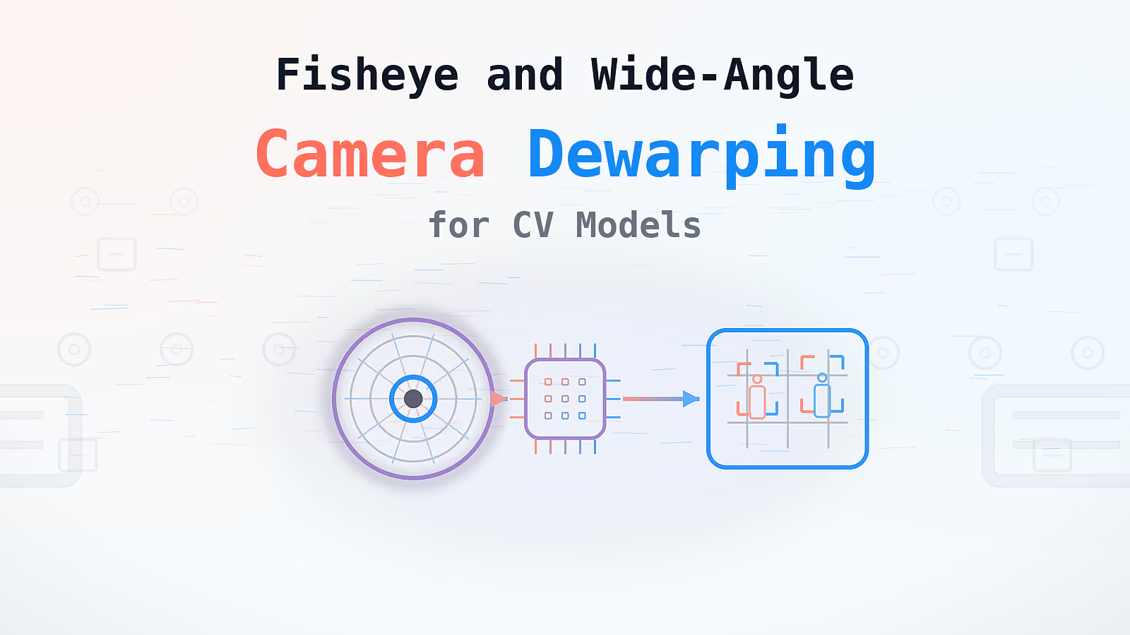
Fisheye dewarping is the geometric correction of wide-angle lens distortion into a flat, usable image, converting a circular, warped fisheye frame into a rectilinear view that looks like it was captured with a standard lens. Most dewarping guides stop there, focused on surveillance monitors and human viewers. This guide answers the question those guides skip entirely: should you dewarp before running a computer-vision model on the footage, or train the model to handle the distortion directly? It is written for CV engineers and surveillance integrators building detection pipelines for security, transit, and industrial inspection, where the answer changes the architecture of the entire system.
Key Takeaways
Fisheye lenses capture images in a circular, warped format, projecting an extremely wide field of view, often 180 degrees or more, onto a flat sensor. The result is a fisheye image where straight lines in the real world curve outward from the center, objects near the edge of the frame appear compressed and stretched, and the entire scene appears to bulge from a central point as if viewed through a glass sphere. Whether that correction runs on the camera module or downstream is a design decision in intelligent hardware development, since dewarping consumes compute and memory bandwidth on every frame.
This distorted, curved appearance is the direct geometric consequence of squeezing a hemisphere of light onto a flat rectangular sensor. A standard rectilinear lens cannot do this at all past a certain field of view, since its projection mathematically approaches infinity as the angle widens. Fisheye lenses solve that problem by using a different mapping function (covered in detail later in this guide), at the cost of this characteristic distortion.
Dewarping converts these circular, distorted images into normal, flat views by applying the inverse of the lens's projection mapping, redistributing the compressed and stretched pixels back into a geometrically correct rectilinear (or other target) projection. The original image, in its raw circular form, is rarely usable directly, either for human viewing or for most computer vision models, which is why dewarping exists as a standard processing step in the surveillance and CV pipeline.
A wide-angle lens creates distortion through its optical projection geometry: to fit a very wide field of view onto a fixed sensor size, the lens must compress the angular space non-linearly, with the compression typically increasing toward the edges of the frame. This is distinct from, but often confused with, perspective distortion.
Perspective distortion is noticeable with wide-angle lenses specifically because subjects near the camera occupy a disproportionately large angular extent relative to subjects farther away, exaggerating the apparent size difference between near and far objects in a way that feels unnatural compared to how the human eye perceives the same scene. A face photographed close-up with a wide-angle lens, for example, will show an enlarged nose and a foreshortened forehead, an effect of the geometry, not a flaw in the lens.
Converging lines are a related but separate phenomenon, caused by camera tilt rather than the lens itself: when a camera is angled upward or downward relative to a scene with vertical lines (a building, a doorway), those lines, which are physically parallel, converge toward a vanishing point in the resulting image. This effect occurs with any lens, but becomes more visually pronounced with wide-angle lenses because more of the converging geometry is captured within the frame. Correcting converging lines (keystone correction) is a distinct operation from fisheye dewarping, covered later in this guide.
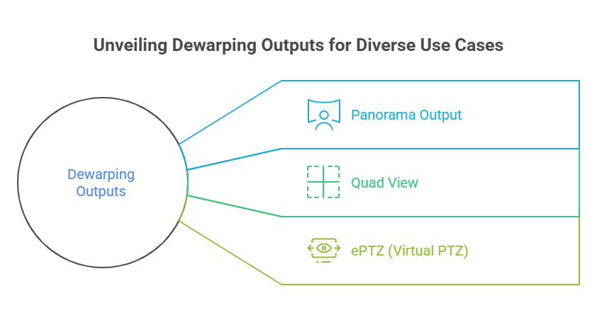
A single fisheye or 360-degree feed can be dewarped into several different output formats simultaneously, each suited to different monitoring and computer-vision use cases. Dewarping provides multiple formats from a 360-degree feed including panorama and quad view, generated from the same underlying source image without requiring multiple physical cameras.
A single wide rectilinear or cylindrical projection unrolling the full circular field of view into one continuous strip, useful for monitoring an entire room or corridor in a single view without the geometric distortion of the raw fisheye frame, though some residual stretching typically remains at the extreme edges of a very wide panorama.
The fisheye frame is split into four separate dewarped regions, each displayed as an independent rectilinear view, effectively simulating four standard fixed cameras from a single fisheye sensor. This is a common monitoring layout for operators reviewing a space from multiple effective viewing angles simultaneously.
Virtual PTZ lets users digitally navigate within the dewarped scene, panning, tilting, and zooming into any region of the original fisheye capture without any physical camera movement, since the entire field of view was already captured and the "movement" is simply a different dewarping window applied to the same source frame. This is a major operational advantage over physical PTZ cameras: multiple operators can independently navigate different regions of the same fisheye feed simultaneously, and nothing outside the current view is ever missed since the full scene was captured at all times.
Outputs include panorama and ePTZ views as the two most common formats requested in surveillance deployments, though the quad view and other custom projection windows remain available from the same underlying fisheye capture whenever a specific monitoring layout calls for them.
The dewarping computation can happen in two fundamentally different places in the pipeline, with materially different implications for system architecture.
Hardware dewarping uses the camera and occupies multiple channels on the NVR. The camera's onboard processor performs the dewarping computation before the video stream ever leaves the device, transmitting an already-corrected view (or several simultaneous views, such as a quad layout) to the recording or analysis system. Because each dewarped output is effectively treated as a separate video stream by the downstream NVR, a single fisheye camera producing four dewarped quad views can consume four channels on the NVR's licensing or channel-count limit, a cost implication that is easy to overlook during procurement.
Software dewarping uses the NVR CPU and requires NVR support for fisheye decoding: the raw, undewarped fisheye stream is transmitted from the camera, and the dewarping computation happens downstream, either on the NVR itself, in a web browser, or in a mobile app. Software dewarping can run on NVRs, web browsers, or mobile apps, which gives significant flexibility: the same raw fisheye stream can be dewarped differently by different consumers (one operator viewing a panorama, another navigating ePTZ) without requiring the camera to generate multiple separate output streams.
Hardware dewarping runs the computation right on the camera itself. Software dewarping happens downstream, on the NVR, in a browser, or on whatever client device is displaying the feed.
That difference in location shapes everything else. Hardware dewarping needs a separate NVR channel for every dewarped view you want to pull out of a single fisheye feed. Software dewarping only needs one channel for the raw stream, since the dewarping happens after the fact.
Bandwidth follows the same logic. With hardware dewarping, each output view gets transmitted as its own stream, so bandwidth usage climbs with every additional view. Software dewarping sends a single raw stream and lets whatever's consuming it handle the dewarp locally.
Flexibility is where the tradeoff really shows up. Hardware dewarping locks you into whatever views you configured on the camera at setup time. Software dewarping lets each consumer pull a different view from the same raw feed, and you can reconfigure those views after the footage was captured, without touching the camera.
None of this comes free on the compute side. Hardware dewarping puts zero additional load on the NVR's CPU, since the camera already did the work. Software dewarping does the opposite: CPU load is required, and it scales up with however many dewarp operations are running at once.
That distinction carries through to storage too. Hardware-dewarped systems typically store footage that's already been dewarped (or raw, depending on how the system is configured). Software-dewarped systems usually store the raw fisheye footage as-is, and only dewarp it at playback time.
Software handles dewarping to save bandwidth and let users pan around recorded footage: because the raw fisheye stream contains the entire field of view in a single feed, storing it raw and dewarping on demand (at playback time, for whatever region an operator wants to review) avoids the bandwidth and storage cost of transmitting and recording multiple separate dewarped streams, while still preserving full post-hoc navigational flexibility across the entire captured scene.
Accurate dewarping depends entirely on accurate calibration. Calibration, specifically the camera's intrinsic parameters and distortion coefficients, is what makes dewarping accurate; without it, the geometric correction is approximate at best and visibly wrong at worst, particularly toward the edges of the frame where distortion is most severe.
The standard calibration procedure involves capturing multiple images of a known calibration pattern (typically a checkerboard) from varied positions and angles within the camera's field of view, then using a calibration algorithm (OpenCV's fisheye calibration module is the common choice) to solve for the camera's intrinsic parameters and distortion coefficients that best explain the observed pattern distortion across all captured images.
Rather than calibrating from scratch for every camera, many manufacturers publish or make available lens profiles, precomputed calibration parameters for a specific camera and lens model, that can be applied directly without requiring an on-site calibration capture. Tools like Lightroom offer lens profiles for correcting distortion in photography contexts, and the same underlying concept (a reusable, lens-specific distortion model) applies directly to CV and surveillance dewarping pipelines, with the caveat that manufacturing tolerances mean a generic profile is always somewhat less accurate than a camera-specific calibration.
Mounting position affects how the image is algorithmically flattened: a ceiling-mounted fisheye camera looking straight down requires a different dewarping geometry (typically optimized for a panorama or quad view radiating outward from the center) than a wall-mounted camera looking across a room at an angle, where the relevant dewarped region is typically a single forward-facing rectilinear window rather than a full radial unwrap. Measuring and recording the camera's mounting height, tilt angle, and roll orientation at installation time is essential input to configuring the dewarping parameters correctly, and should be documented as part of the installation record so it can be reproduced if the dewarping configuration ever needs to be regenerated.
At its core, dewarping maps the distorted pixels back to a proper perspective using algorithms that invert the lens's forward projection function. The camera's lens applies a forward mapping (from a real-world angle to a pixel position on the distorted sensor image); dewarping applies the corresponding inverse mapping (from a distorted pixel position back to its correct position in a flat, undistorted projection).
Geometric algorithms correct circular distortion by mapping it back to a flat plane, computing, for every pixel in the desired output image, which pixel (or, more precisely, which interpolated location) in the original distorted source image corresponds to it. This pixel-by-pixel correspondence is the fundamental computation underlying every dewarping implementation, regardless of whether it runs in hardware, as an FFmpeg filter, or as custom code, and regardless of which specific projection model is used to define the geometric transform.
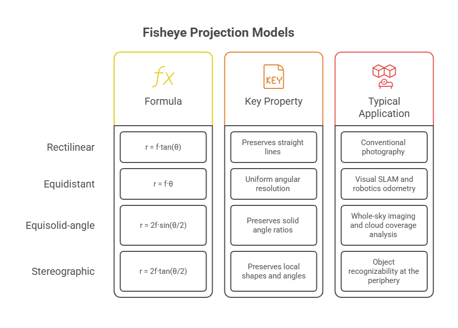
Fisheye lenses do not all use the same optical projection, and understanding which projection a given camera uses (or assumes) is essential to building an accurate dewarping transform.
Rectilinear projection (the standard, non-fisheye case) follows r = f·tan(θ), where r is the distance from the image center, f is the focal length, and θ is the angle of incidence of the light ray. This projection preserves straight lines as straight lines, which is why standard photography looks geometrically "normal," but the tangent function approaches infinity as θ approaches 90 degrees, mathematically preventing rectilinear lenses from capturing a field of view anywhere near 180 degrees.
Equidistant projection follows r = f·θ, a direct linear mapping between angle and image radius. This gives uniform angular resolution across the entire field of view, meaning every pixel subtends the same angular extent regardless of its position in the frame, which makes equidistant fisheye lenses a strong choice for applications like visual SLAM and robotics odometry, where consistent feature tracking from the center to the edge of the frame is important.
Equisolid-angle projection follows r = 2f·sin(θ/2). This projection preserves solid angle ratios, meaning equal areas in the real-world scene map to equal areas on the sensor, which is the property that makes equisolid lenses well suited to applications like whole-sky imaging and cloud coverage analysis, where area measurement matters more than preserving local shape.
Stereographic projection follows r = 2f·tan(θ/2). This projection is conformal, meaning it preserves local shapes and angles even though it distorts overall scale across the frame, which means objects at the extreme edges of a stereographic fisheye frame retain their recognizable shape better than under the other projection models, at the cost of more pronounced area distortion (objects near the edge appear larger relative to their true size than under equidistant or equisolid mapping).
This choice sets your calibration work, your training data and your compute budget on the device. We benchmark both paths on your own camera footage before you commit.
Decide dewarp or train on distortion with real numbers
Projection models comparison
Rectilinear projection follows the formula r equals f times tan(θ). It preserves straight lines, which makes it the standard choice for conventional photography. The catch: it physically cannot exceed a field of view around 180 degrees, since the math breaks down as theta approaches 90 degrees.
Equidistant projection uses r equals f times θ. What it preserves is uniform angular resolution across the frame, meaning equal angular steps map to equal pixel distances regardless of position in the image. That property is exactly why it shows up so often in SLAM and robotics odometry work, where consistent angular mapping matters more than natural-looking geometry.
Equisolid-angle projection, calculated as r equals 2f times sin(θ/2), preserves equal-area mapping instead. A patch of sky covering a fixed solid angle takes up the same pixel area no matter where it falls in the frame. That property is what makes this projection the right fit for sky imaging and general area or coverage analysis.
Stereographic projection, r equals 2f times tan(θ/2), preserves local shape, or conformality, meaning small shapes stay recognizable even out toward the edges of a heavily distorted frame. That's the specific advantage that makes it useful when object recognizability at the periphery of the image actually matters for the task.
Most consumer and security fisheye cameras are manufactured closer to an equidistant or equisolid model, though manufacturing tolerances mean real lenses rarely match any of these idealized projections perfectly. More advanced calibration approaches (the Kannala-Brandt polynomial model is a widely used example) fit a more flexible function to the camera's actual measured distortion rather than assuming it conforms exactly to one of the four classical projection formulas, which is generally the more accurate approach for production CV pipelines where geometric precision matters.
Once the geometric mapping between distorted and corrected pixel positions is known, the actual dewarping operation requires resampling the source image at the computed (often non-integer) source coordinates for every destination pixel, a process called remapping, and that resampling requires an interpolation method.
Nearest-neighbor interpolation simply takes the value of the closest source pixel, the fastest method but the lowest quality, producing visible blocky artifacts, particularly in regions of high distortion where source pixels are stretched significantly. Bilinear interpolation averages the four nearest source pixels weighted by distance, a reasonable quality-speed compromise suitable for most real-time CV preprocessing applications. Bicubic interpolation uses a larger 4x4 neighborhood and produces smoother results with less aliasing, at higher computational cost, generally reserved for applications where output image quality for human viewing matters more than processing speed.
A naive pixel-by-pixel remapping implementation in pure Python, iterating over every output pixel individually, performs very poorly: pure Python loops carry substantial per-operation interpreter overhead that compounds across the millions of pixel operations a typical frame requires. A vectorized NumPy implementation, which performs the same remapping operation across the entire image array at once using NumPy's underlying C implementation, is dramatically faster, commonly cited as well over an order of magnitude improvement over the equivalent naive Python loop on comparable hardware (Grosjean, benchmark comparison of six dewarping implementations, 2026). GPU-based remapping (via OpenCV's CUDA-accelerated remap function, or a custom GPU kernel) is faster still for high-resolution, high-frame-rate pipelines, though the overhead of transferring frame data to and from GPU memory needs to be accounted for in the total pipeline latency, particularly for single-camera applications where that transfer overhead is not amortized across many parallel streams.
For a fixed camera (one that does not move or change zoom after calibration, which describes the overwhelming majority of security and industrial CV deployments), the pixel-to-pixel mapping between distorted and corrected coordinates is constant across every frame. This means the expensive part of the computation, deriving the per-pixel source coordinates from the projection model and calibration parameters, only needs to happen once, at setup time, producing a lookup table (a remap map) that can then be applied to every subsequent frame with a single, highly optimized remap operation. This is the fact that resolves most performance objections to dewarping before detection: real-time dewarping for a fixed camera costs almost nothing per frame, because the geometric computation has already been done in advance.
FFmpeg v360 filter. FFmpeg supports dewarping via its v360 filter, which handles conversion between a wide range of input and output projections (fisheye, equirectangular, flat/rectilinear, and others) directly from the command line or as part of a larger FFmpeg processing pipeline.
bash
ffmpeg -i input.mp4 -vf "v360=fisheye:flat:ih_fov=180:iv_fov=180:pitch=0:yaw=0:w=1280:h=720" output.mp4
This example command takes a 180-degree fisheye input and outputs a flat (rectilinear) projection at 1280x720, centered with no pitch or yaw offset. The pitch, yaw, and roll parameters can be adjusted to extract a different region of the source fisheye frame, supporting the ePTZ-style navigation covered earlier in this guide.
OpenCV remap example (Python).
python
import cv2
import numpy as np

# map_x, map_y are precomputed once from calibration parameters
# and the chosen projection model (see Projection Models section)
def dewarp_frame(frame, map_x, map_y):
    return cv2.remap(
        frame, map_x, map_y,
        interpolation=cv2.INTER_LINEAR,
        borderMode=cv2.BORDER_CONSTANT
    )

# Applied per frame in a video loop:
# dewarped = dewarp_frame(raw_frame, map_x, map_y)
Because map_x and map_y are computed once (per the precomputation point made above) and reused for every frame, the per-frame cost of this operation is a single, highly optimized cv2.remap call, not a re-derivation of the geometric transform.
Custom optimized C++ pipeline outline. For the highest-throughput, lowest-latency deployments (multi-camera edge systems with strict frame budgets), a custom C++ implementation typically follows this structure: precompute the remap lookup tables once at startup or calibration time; load each incoming frame directly into GPU or SIMD-aligned memory; apply the remap using a vectorized or GPU-accelerated operation equivalent to OpenCV's remap but integrated directly into the existing capture and inference pipeline to avoid unnecessary memory copies between processing stages; pass the dewarped frame directly to the downstream detection model without an intermediate encode/decode step. With dewarping this lean, the downstream detector usually dominates the frame budget, which is where model quantization for edge inference pays off.
FFmpeg processes 1024 frames in 208 seconds in one published benchmark using the command-line v360 filter on standard CPU hardware (Grosjean, 2026), a measured example specific to that test configuration (resolution, output format, and hardware were held constant in that test) rather than a universal performance figure; actual throughput for any specific deployment should be benchmarked directly rather than assumed from a single published number.
This is the question that surveillance-focused dewarping guides almost never address, and it is the core engineering decision this guide exists to clarify.
Distortion does not only shift bounding boxes. Keypoint models degrade in the same way, so any pipeline that runs human pose estimation and action recognition on a wide-angle feed has to decide whether the skeleton is fitted on the raw frame or on the dewarped one.
Objects near the center of a fisheye frame are relatively undistorted and close to their natural appearance. Objects toward the edge of the frame are significantly stretched and compressed by the lens projection, changing their apparent shape, aspect ratio, and effective resolution in ways that a detection model trained on standard rectilinear imagery has never seen. A person standing near the edge of a fisheye frame may appear elongated, curved, or compressed in a way that a standard object detector, trained overwhelmingly on rectilinear photography, fails to recognize reliably.
Dewarp-then-detect applies the geometric correction before passing the frame to the detection model. This gives the model clean, familiar geometry, closely matching the rectilinear imagery most detection models were originally trained on, which typically produces the best accuracy with the least amount of custom model training required. The trade-offs: there is an additional processing step in the pipeline (though, per the precomputation point above, this is cheap for a fixed camera), and dewarping a wide field of view into a single flat output frame can introduce information loss or extreme stretching at the very edges of that output, particularly for wide fields of view dewarped into a single flat projection, sometimes requiring multiple overlapping dewarped views rather than one to fully preserve detail across the original field of view.
Train the model on distorted frames skips the dewarping preprocessing step entirely, instead training (or fine-tuning) the detection model directly on raw fisheye imagery, so the model itself learns to recognize objects despite the distortion. This avoids the preprocessing compute cost and any information loss from the dewarping transform itself, but requires a training dataset that is genuinely representative of fisheye-distorted footage, which is far less abundant than standard rectilinear training data, and the model must independently learn the geometric relationship between object distortion and its position in frame, a relationship that dewarping would otherwise resolve explicitly through the geometric transform.
Several scenarios favor skipping dewarping. When compute is genuinely constrained and a fixed-camera precomputed remap is for some reason not available (a rare case, but possible for cameras with adjustable zoom or pan), the preprocessing overhead may not be justified. When sufficient fisheye-representative training data already exists or can be generated (synthetically distorting a standard dataset, for example, using the same projection model as the deployment camera), training directly on distorted frames avoids the dewarping step's edge-distortion trade-offs entirely. When the detection task is concentrated near the center of the frame, where distortion is minimal, the accuracy benefit of dewarping may not justify the engineering effort at all.
Overhead fisheye cameras are the standard mount for counting people in a cabin or on a platform, and those pipelines often score the raw circular frame rather than a dewarped view. If the deployment target is passenger counting and crowd density estimation, test both paths before committing the remap step to the edge compute budget.
As established in the Remapping section, precomputed maps make dewarping cost almost nothing per frame for a fixed camera, which removes the strongest argument against dewarping (compute overhead) for the overwhelming majority of security and industrial deployments where cameras are mounted in a fixed position. This is the practical recommendation for most production systems: dewarp using a precomputed map, then run a standard, well-supported detection model on the resulting clean geometry, reserving the train-on-distorted approach for cases with a specific reason to avoid the dewarping step.
For detection accuracy at small object scales, which compounds with the edge-distortion problem since small or distant objects near the frame edge suffer both the small-object detection challenge and the geometric distortion challenge simultaneously, see small object detection with SAHI. For the broader CCTV threat-detection context where this distortion-handling decision most commonly arises in practice, see edge AI CCTV threat detection.
The single most effective way to avoid converging-line distortion is preventing it at the source: mounting the camera with a level roll axis (no unintended tilt left-to-right) and a deliberate, documented pitch angle (rather than an arbitrary one), minimizes the perspective correction that any downstream processing needs to perform.
Where camera tilt is unavoidable (a ceiling or high-wall mount angled down toward a scene, for example), keystone correction applies a perspective transform that counteracts the convergence of vertical lines caused by that tilt, distinct from and typically applied in addition to the fisheye-specific dewarping covered throughout the rest of this guide.
Both fisheye dewarping and keystone correction can leave irregular, non-rectangular regions at the edges of the corrected output (black or undefined pixels where the transform has no valid source data). Cropping to a clean rectangular region after applying these geometric corrections, rather than before, ensures the final output frame is uniformly well-defined across its entire area, which matters both for downstream CV model input consistency and for clean presentation to a human operator.
Dewarped output frequently shows a quality gradient: sharp, high detail near the center of the original fisheye frame (where the lens had the least distortion to begin with), degrading toward softer, less distinct detail near the edges of the dewarped output, an artifact of stretching a smaller number of original source pixels across a larger area in the corrected image. This is a fundamental consequence of the geometry, not a correctable processing error, and should be accounted for explicitly in camera placement and resolution planning rather than treated as a bug to be fixed in post-processing.
When a single fisheye source feeds multiple simultaneous outputs (a panorama for one operator, an ePTZ window for another, a detection pipeline for a third), each output draws from the same finite pool of original sensor pixels. A high-resolution sensor (8MP or higher is increasingly standard for fisheye security cameras) provides more headroom across simultaneous outputs, but the resolution budget should still be planned explicitly: a detection pipeline targeting small or distant objects near the frame edge needs more native sensor resolution in that region than a simple wide-area panorama intended only for general human situational awareness would require.
A published comparison of six different dewarping implementations, command-line FFmpeg, native Python (pure loops, no libraries), vectorized NumPy, OpenCV (both Python and C++ bindings), and a custom optimized C++ implementation, provides a useful reference point for the performance and complexity trade-offs across approaches (Grosjean, 2026). The comparison covered execution time, memory usage, and implementation complexity across all six approaches, benchmarked on a fixed test configuration of resolution, output format, and hardware.
General performance and accuracy patterns observed across published benchmarks:
Memory usage follows a related pattern: pure Python and naive implementations often carry higher peak memory overhead from intermediate data structures, while vectorized and GPU-accelerated approaches tend to operate more efficiently within a fixed, predictable memory budget, an important consideration for embedded edge deployments with limited RAM.
InTechHouse's experience handling edge distortion in a delivered vision system grounds these general benchmark patterns in a specific applied context: a production deployment where detection accuracy at the frame periphery was a hard requirement, not just a nice-to-have, because the safety-relevant objects of interest could appear anywhere in the camera's field of view, including the heavily distorted edge regions where generic detection models perform worst without correction.
InTechHouse case study: Frame-edge detection accuracy in a wide-angle CCTV deployment for public transport safety
InTechHouse addressed wide-angle lens distortion in a CCTV-based vision system developed for a public transport manufacturer, where cabin cameras using wide-angle lenses to maximize coverage from a single mounting position needed to support reliable detection across the entire field of view, including the heavily distorted regions near the frame edges where passengers and objects most often appeared given typical cabin geometry.
The team adopted a dewarp-then-detect architecture rather than training the detection model directly on distorted frames, given the fixed, unmoving mounting position of the onboard cameras: this meant the pixel remap could be precomputed once per camera at installation and calibration time, making the dewarping step computationally negligible for every subsequent frame processed in real time.
Detection accuracy at the frame edges, validated specifically in those peripheral regions rather than relying on an aggregate accuracy figure that could mask edge-region weakness, improved measurably relative to running the same detection model on raw, undewarped fisheye frames, confirming that the precomputed dewarping step was solving a genuine accuracy problem rather than adding unnecessary pipeline complexity.
Read also:
Finalize the camera's physical mounting position, tilt, and roll before running any calibration capture, since calibration parameters and the resulting dewarping configuration are specific to that exact mounting geometry; recalibration is required if the camera is later remounted or its orientation changes. Mounting discipline matters even more in multi-sensor rigs, since camera, LiDAR and radar fusion relies on extrinsic calibration between every sensor pair.
Use a clear, properly lit calibration pattern capture covering the camera's full field of view, including the heavily distorted edge regions, to ensure the resulting calibration is accurate across the entire frame, not just near the optically cleaner center.
Validate the dewarping configuration in both real-time operation and on recorded footage, since some deployment architectures (particularly software dewarping applied at playback time, covered earlier) can behave differently between the two contexts, and both need to perform correctly for a production deployment.
Where the target platform supports GPU-accelerated remapping (CUDA on NVIDIA edge hardware, for example) and the deployment involves multiple concurrent camera streams, enabling that acceleration is typically the most effective single performance optimization available, particularly relative to the marginal gains available from further optimizing a CPU-only software implementation.
A dewarping operation that is fast in isolated benchmarking can still bottleneck a real pipeline if frame capture, format conversion, or the handoff to the detection model introduces overhead the isolated benchmark did not account for; profile the complete pipeline, not just the dewarp call.
Unless the deployment specifically requires runtime recalibration (a PTZ-capable fisheye camera with adjustable zoom, for instance), default to the precomputed remap-map approach, which is both simpler to implement correctly and dramatically cheaper per frame than recomputing the geometric transform on the fly.
OpenCV's fisheye calibration and remap modules provide a complete, well-documented Python and C++ toolkit for calibration, map generation, and per-frame dewarping. FFmpeg's v360 filter handles a broad range of input and output projection conversions directly from the command line, well suited to batch processing of recorded footage or simple pipeline integration without custom code.
Several published computer vision datasets specifically include fisheye or wide-angle captures for benchmarking detection and calibration methods under realistic distortion conditions, useful both for validating a dewarping pipeline and, where the train-on-distorted approach is chosen instead, for training a detection model directly on representative distorted imagery.
OpenCV's documentation includes standard checkerboard pattern generators sized appropriately for camera calibration; printing a pattern at a known, precisely measured physical size is essential, since the calibration algorithm relies on that known real-world scale to solve for the camera's intrinsic parameters accurately.
This is a practical resource list rather than an exhaustive survey; teams implementing a production dewarping pipeline should expect to validate their chosen tools and methods directly against their specific camera hardware and deployment conditions rather than assuming results transfer directly from a different camera model or projection type.
We deploy detection on wide-angle camera fleets in transit and industrial sites, with the remap precomputed and the accuracy loss measured rather than assumed. Ask for our numbers.
See how we build fisheye vision pipelines that run at the edge
Not sure where to start? We work with companies at every stage, from early ideas to enterprise-level builds. A 30-minute call can save you months of guesswork.
Fisheye dewarping is the geometric correction process that converts a distorted, circular fisheye image into a flat, rectilinear (or other target projection) view, undoing the optical distortion introduced by a wide-angle lens. It works by mapping each pixel in the distorted source image to its correct position in the corrected output, based on the camera's known projection model and calibration parameters.
The standard approach calibrates the specific camera to determine its intrinsic parameters and distortion coefficients, then computes a pixel remap (a lookup table mapping distorted source coordinates to corrected output coordinates) using a projection model such as equidistant, equisolid, or stereographic. For a fixed-position camera, this remap is computed once and then applied to every subsequent frame using an optimized remap operation (available in OpenCV, FFmpeg's v360 filter, or a custom implementation), making per-frame correction computationally cheap.
In most cases, yes, particularly for fixed cameras where the dewarping computation can be precomputed and applied at near-zero per-frame cost. Dewarping before detection gives the model clean, familiar rectilinear geometry, typically improving accuracy without requiring the model itself to be retrained on distortion-specific data. The alternative, training the detection model directly on distorted frames, is worth considering primarily when sufficient fisheye-representative training data is already available or when the detection task is concentrated near the frame center where distortion is minimal.
Yes, and the effect is most pronounced at the frame periphery, where wide-angle lens projection stretches and compresses objects most severely. A standard object detection model, trained predominantly on rectilinear photography, generally performs worse on raw fisheye frames than on the equivalent dewarped imagery, particularly for objects near the edge of the field of view, which is exactly where distortion is most extreme and where safety-relevant objects in a wide-coverage camera deployment most often appear.
For a fixed camera, very little. The expensive part of dewarping, deriving the per-pixel geometric mapping from the camera's calibration parameters and chosen projection model, only needs to be computed once and stored as a lookup table. Applying that precomputed map to each subsequent frame is a single, highly optimized remap operation (available as a built-in, GPU-accelerable function in OpenCV), making real-time dewarping for a static camera computationally negligible relative to the cost of the downstream detection model itself.
Damian Ledziński, PhD Eng., is an Applied Artificial Intelligence Expert and an Assistant Professor at Bydgoszcz University of Science and Technology. He has over 15 years of academic, research, software-engineering, and technology-development experience.
His work focuses on applying artificial intelligence, machine learning, deep neural networks, and data science to complex real-world systems. His principal research and engineering interests include autonomous unmanned aerial vehicles, drone navigation and swarm intelligence, biomedical engineering, medical signal and image analysis, predictive modeling, industrial IoT, and intelligent water-management systems.
Damian has contributed to multidisciplinary R&D initiatives including AI-assisted medical diagnostics, a Polish ventilator prototype, autonomous indoor drone systems for warehouse inventory, AI-supported water-consumption analysis, virtual medical assistants, and intelligent systems combining embedded devices with machine-learning models.
He is the author or co-author of more than 30 scientific publications. His work has appeared in international scientific publications covering artificial intelligence, biomedical engineering, signal analysis, autonomous systems, environmental monitoring, and data-driven infrastructure.
Damian is a co-creator of academic programs in Engineering in Medicine, AI in Medicine, and Data Science at Bydgoszcz University of Science and Technology. He combines scientific research with hands-on implementation, translating experimental AI methods into deployable technology. He writes about applied AI, machine learning, predictive analytics, autonomous UAV systems, AI in medicine, biomedical signal processing, industrial IoT, and intelligent models in real-world systems.
Damian Ledziński's academic profiles:
https://orcid.org/0000-0003-0796-4390
https://wtie.pbs.edu.pl/pl/pracownik/damian-ledzinski
https://www.researchgate.net/profile/Damian-Ledzinski
https://scholar.google.pl/citations?user=AlQpPB0AAAAJ&hl=pl
https://ludzie.nauka.gov.pl/ln/profiles/DN6pHXU6KZm/publications/f83a8833-6060-4fae-8628-3dbf57661394
From first prototype to production, our engineers can help you scope it, build it and get it certified.
This initial conversation is focused on understanding your product, technical challenges, and constraints.
No sales pitch - just a practical discussion with experienced engineers.
Share a few details about your product and context. We’ll review the information and suggest the most appropriate next step.