
Sensor fusion edge AI is the combination of data from multiple sensors (camera, LiDAR, radar) processed in real time on an embedded compute unit, without cloud connectivity, which is the core edge AI vs cloud AI trade-off. No single sensor is sufficient for reliable perception: cameras lack depth, LiDAR struggles in heavy rain, radar lacks spatial resolution. Fusion compensates for each sensor's individual weaknesses by cross-referencing what each one sees. This guide covers how that fusion works at the edge, why it runs on-device rather than in a data center, and why it matters for safety in automotive, transit, and industrial deployments.
Key Takeaways
Sensor fusion combines data from multiple sensors to perceive the environment more reliably and completely than any single sensor can. In a perception pipeline for a vehicle or safety system, that means taking sensor data from cameras (rich color and texture), a LiDAR sensor (precise 3D point cloud), and radar sensors (velocity and all-weather range) and producing a unified model of the environment: what objects are present, where they are, how fast they are moving, and how confident the system is in each estimate.
Edge AI provides the compute platform for real-time computer vision on embedded hardware, running that pipeline on-device. Processing locally means the perception output is available within the latency budget of the safety application (typically 10–33 ms for frame-by-frame vehicle decisions) without any network round-trip. For autonomous driving and transit safety, that latency is not a preference; it is a hard constraint.
Each sensor has a characteristic weakness that the others compensate for. Cameras provide accurate object recognition and classification but fail in low light and cannot directly measure distance. LiDAR provides precise 3D geometry but degrades significantly in heavy precipitation and can be occluded by dirt or ice on the sensor window. Radar sensors penetrate rain, fog, and darkness and measure velocity directly through the Doppler effect, but their spatial resolution is coarse: they can detect that something is present and moving at 15 m/s, but they cannot reliably distinguish a pedestrian from a bicycle at close range. Combining data from these various sensors compensates for individual sensor weaknesses, enhancing reliability in adverse conditions that would defeat any single sensor.
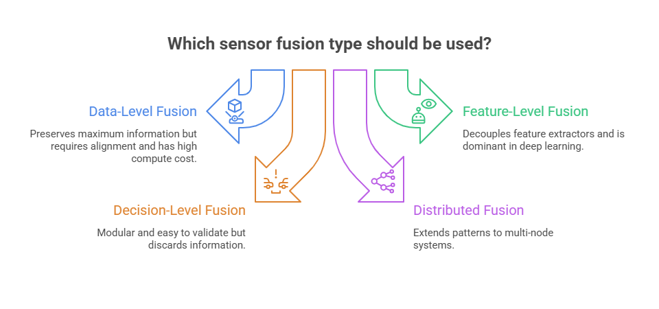
Sensor fusion architectures differ in where in the processing pipeline the combination happens. The choice between types is a design decision that affects latency, compute cost, accuracy, and system complexity.
Data-level fusion combines raw sensor data (the camera frame and the LiDAR point cloud) before any feature extraction. This preserves the maximum amount of information and gives a learned model access to raw cross-sensor correlations, but requires solving the alignment problem (projecting 3D LiDAR points onto the 2D camera image plane) before any processing, and the compute cost scales with raw data volume.
Feature-level fusion extracts features from each sensor independently (bounding box proposals from the camera, 3D object proposals from the LiDAR), then merges them in a shared feature space. This is the dominant approach in modern deep-learning fusion networks because it decouples the per-sensor feature extractors (which can be optimized independently) from the fusion layer. Most production-level camera lidar fusion systems use this pattern.
Decision-level fusion runs separate detection pipelines on different sensors and combines their outputs using a voting, weighting, or Bayesian combination rule. This pattern is the most modular and the easiest to validate independently: each sensor's pipeline can be tested in isolation, and the combination logic is explicit.
For safety-critical systems where each component must have a traceable failure mode, and where explainable AI for operator alerts has to justify every warning, decision-level fusion simplifies the safety case. The trade-off is that information is discarded at each independent decision step before the combination.
Distributed fusion and decentralized architectures extend these patterns to multi-node systems where fusion happens across physically separate processing units. In an in-vehicle system, this typically means each sensor module has its own preprocessing CPU, and a central edge AI compute unit aggregates the pre-processed outputs.
Kalman filter variants are the classical backbone of sensor fusion for state estimation. The standard Kalman filter is optimal for linear systems with Gaussian noise. Most real-world sensor fusion problems are non-linear (object motion on a curved track, sensor measurement geometries), which requires the Extended Kalman Filter (EKF) or the Unscented Kalman Filter (UKF).
The EKF linearizes the non-linear system dynamics around the current state estimate using a first-order Taylor expansion. It is computationally efficient but introduces linearization error when the system is highly non-linear. The UKF propagates a set of carefully chosen sigma points through the non-linear functions, producing a better approximation of the state distribution without linearization. In published benchmarks on LiDAR-radar fusion for vehicle tracking, the UKF achieves 24% lower average RMSE than EKF across all tracked state variables (Farag, ResearchGate, 2021). The cost is higher computational overhead, which is a real constraint on resource-constrained edge hardware.
Fusing LiDAR and radar using a UKF achieves high-precision simultaneous position and velocity tracking that neither sensor can deliver independently (Jiangsu University, 2021). LiDAR provides accurate position but poor velocity estimation; radar provides accurate velocity but coarse position. The UKF combines both to produce accurate results on both dimensions simultaneously, which is the primary engineering reason radar retains a role even in LiDAR-heavy autonomy stacks.
Particle filters represent the state distribution as a set of weighted samples (particles) that propagate through the system model. They handle highly non-linear, non-Gaussian distributions that Kalman variants cannot represent well. The trade-off is compute cost: accurate particle filters require hundreds to thousands of particles, making them impractical for high-frequency sensor fusion on constrained hardware. They are used in low-frequency localization tasks (global pose estimation) rather than object-level perception fusion.
Deep learning fusion approaches have overtaken classical filters for perception accuracy on standard datasets. Models like BEVFusion (MIT, 2022) and TransFusion operate in the Bird's Eye View (BEV) space, fusing camera and LiDAR features through attention mechanisms that learn the cross-modal relationships directly from data. CLF-BEVSORT achieves a HOTA score of 77.26% on the KITTI Car class for multi-object tracking, surpassing earlier fusion methods (MDPI Sensors, 2024). These deep-learning approaches produce more accurate decisions than classical filters on well-represented scenarios, but they require more inference compute and are harder to analyze for corner-case failure modes than explicit Kalman-based pipelines. For safety-critical deployments, the choice between classical and learned fusion often depends on the certification requirements of the applicable safety standard.
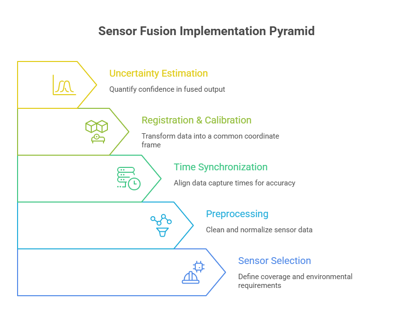
Getting sensor fusion working in a lab is straightforward. Getting it to work reliably in field deployment is where most projects discover their real challenges. The steps below are ordered by the dependencies they create: each step is a prerequisite for the next.
1. Sensor selection and placement. Define the coverage requirements (forward, 360°, or combined), select sensor types that cover the required detection range and work in the expected environmental conditions, and place sensors to minimize occluded zones. Camera-LiDAR overlap should cover the primary detection zone. Radar placement should be co-located with the forward camera for velocity augmentation.
2. Preprocessing and denoising. Before fusion, each sensor stream requires cleaning. LiDAR point clouds are filtered for ground points, outliers, and motion artifacts. Camera frames are pre-processed for lens distortion correction (dewarping for fisheye lenses) and normalization. Radar returns are filtered to remove static clutter (guardrails, overhead structures) that would otherwise produce false detections. This preprocessing runs on the edge device's CPU or dedicated ISP before the fusion pipeline.
3. Time synchronization. This is where field deployments fail. Camera, LiDAR, and radar operate at different frequencies (camera at 30 FPS, LiDAR at 10–20 Hz, radar at 10–20 Hz) and have different processing delays. Fusing data that was captured at different physical times introduces spatial error proportional to the relative motion between capture and fusion. Time synchronization requires hardware triggering (the camera frame is exposed when the LiDAR sweep is at the center of the camera FOV) or software interpolation with precise timestamping. nuScenes achieves this through synchronized hardware triggering, which is one reason it became the dominant benchmark dataset for real time processing validation. Without hardware-level time synchronization, a vehicle moving at 50 km/h moves 1.4 meters in 100 ms, which is enough displacement to corrupt an object's fused position significantly.
4. Sensor registration and calibration. Sensor registration transforms all sensor data into a common coordinate frame. The LiDAR-to-camera extrinsic calibration (the 6-DOF transform between the LiDAR frame and each camera frame) must be accurate to sub-centimeter precision for useful projection of 3D points onto 2D images. This calibration is performed using a checkerboard or target-based procedure before deployment and must be re-validated after any mechanical change to the sensor mounting. Calibration drift in the field (caused by vibration, thermal cycling, or minor physical impacts) is a real maintenance failure mode. Systems that do not monitor calibration accuracy will degrade silently.
5. Uncertainty estimation and validation. The fused output should carry a confidence measure, not just a point estimate. Kalman-based fusion propagates uncertainty explicitly through the covariance matrix. Deep-learning approaches require post-hoc calibration of confidence scores (temperature scaling, conformal prediction) to produce reliable uncertainty estimates. Robust and reliable uncertainty estimation is essential for safety systems that need to know when to trigger a fallback behavior.
A 33 ms perception loop leaves no room for a cloud round trip or a badly scheduled fusion step. We build camera, LiDAR and radar pipelines that meet the latency and power budget of the hardware you actually ship.
Get your perception stack inside the latency budget
The detection output of a fused perception system is richer than any single-sensor system can produce:
LiDAR-to-camera projection overlays the 3D point cloud onto the camera image using the extrinsic calibration transform. Each LiDAR return in the camera's frustum is projected to a pixel location, associating depth measurements with visual features. This allows the 2D object detector running on the camera image to be augmented with precise 3D distance information from LiDAR, producing 3D bounding boxes with depth that camera-only systems cannot generate. The camera provides accurate object classification; the LiDAR provides the metric geometry. The combination is what enables reliable 3D object detection at range.
Radar provides direct radial velocity measurements through the Doppler effect, which camera and LiDAR cannot measure directly. Fusing radar data into the object tracking pipeline gives each tracked object a velocity estimate from a physics-based measurement rather than from frame-differencing of position estimates. This matters most for collision risk assessment: knowing that an object is approaching at 12 m/s is more valuable than inferring it is moving from two consecutive position estimates.
ADAS sensor fusion of cameras, radar, and LiDAR provides a 360-degree view of vehicle surroundings by combining sensors with overlapping and complementary coverage zones. A camera suite covering forward, rear, and side views combined with a 360° LiDAR and corner radars produces a perception field with no blind spots in the primary detection zone.
Evaluation metrics for multimodal detection: mAP (mean Average Precision) at IoU 0.5 and 0.7 thresholds, NDS (nuScenes Detection Score) for multi-class multi-range evaluation, HOTA (Higher Order Tracking Accuracy) for multi-object tracking, and RMSE for state estimation accuracy. Tracking metrics such as HOTA carry over to people-centric tasks too, including the accuracy validation behind AI passenger counting.
Recommended datasets for multimodal training: nuScenes (6 cameras, 1 LiDAR, 5 radars, 1,000 scenes), KITTI (2 cameras, 1 LiDAR), Waymo Open Dataset (5 cameras, 1 LiDAR). See the Appendix for full dataset details.
For safety systems, sensor fusion is not about marginal accuracy improvement. It is about operating reliably when one sensor fails or degrades. A single sensor is a single point of failure. A fused system with appropriate redundancy continues operating if one sensor is compromised.
Each sensor has environment-specific blind spots. Cameras fail in darkness, direct glare, and heavy fog. LiDAR accuracy degrades in heavy rain and snow, which attenuates the laser returns and fills the point cloud with noise. Radar sees through rain and fog and measures velocity reliably, but its spatial resolution is insufficient to classify small objects or pedestrians at close range without camera context. In a complex environment where all three of these conditions may be encountered, a system relying on any single sensor will have scenarios where it cannot operate safely.
Fusion adds redundancy that keeps a system operating during sensor degradation. If the LiDAR window is dirty and range is degraded, the camera-radar pair continues to provide object detection and velocity. If the camera is blinded by direct sunlight on a wet road, LiDAR-radar fusion maintains 3D position and velocity tracking. The fused system's confidence estimate drops (uncertainty increases), which triggers appropriate safety responses (such as increased following distance or reduced operating speed) rather than catastrophic failure.
Sensor fusion enhances safety features like automatic emergency braking by providing a more reliable triggering condition: a single-sensor false alarm might fire the brakes unnecessarily; a fused system that requires multi-sensor confirmation before triggering reduces false activation rates while maintaining high true-positive detection rates. See AI collision avoidance for trams and light rail for a deployment example where this fusion architecture was applied to a safety-critical rail application.
ADAS sensor fusion covers the full SAE autonomy stack from Level 2 (driver assistance with camera-based lane keeping and radar-based adaptive cruise) through Level 4 (full automation in defined operational design domains). The perception pipeline for Level 2–3 autonomy uses a forward-facing camera lidar fusion for object detection and tracking, plus radar for closing-speed measurement. Level 4 perception systems add 360° coverage, higher-resolution LiDAR, and corner radars to eliminate blind spots entirely. Sensor fusion is essential for autonomous vehicles because no single modality provides the combination of range, resolution, and all-weather reliability needed for full autonomy.
A tram runs on a fixed track and cannot steer around an obstacle; the only intervention is braking. Camera-LiDAR fusion provides the forward detection pipeline: the camera classifies the obstacle type (person, vehicle, debris) while the LiDAR provides the precise distance needed to calculate whether braking can prevent a collision. This is a demanding real world application because the tram operates in shared urban space with pedestrians and road traffic, at speeds where the stopping window is measured in tens of meters.
Industrial applications use sensor fusion to detect anomalies and predict failures in equipment, monitor safety zones around collaborative robots, and verify that protective areas are clear before automated machinery cycles. An overhead LiDAR covering a robot work cell, combined with cameras at each access point, provides redundant confirmation that no person is within the danger zone. Industrial IoT applications combine sensor data from pressure, temperature, vibration, and optical sensors to detect failure signatures that no single sensor captures alone.
Mobile robots and autonomous guided vehicles (AGVs) in warehouses and factories use camera-LiDAR-radar fusion for navigation and obstacle avoidance in dynamic environments. The robotics stack includes SLAM (simultaneous localization and mapping) as well as perception, both of which benefit from multi-sensor fusion.
Redundancy requirements for safety validation: safety-critical applications at SIL 2 or above typically require redundant sensing with independent failure modes. Camera and LiDAR are both susceptible to optical blockage (a dirty lens or window affects both), while radar is not, making radar a natural independent failure mode for redundancy in automotive and rail safety contexts. ISO 26262 (automotive) and EN 50126/50128/50129 (rail) define the framework; the sensor architecture must be designed to demonstrate the required redundancy.
The compute requirements for real-time sensor fusion at the edge depend on the sensor count, model complexity, and frame rate. A minimal system (1 camera, 1 LiDAR, 30 FPS object detection) requires 20–50 TOPS of sustained AI inference. A full 360° multi-camera, multi-LiDAR system can require 200+ TOPS.
NVIDIA Jetson AGX Orin (up to 275 TOPS, 15–60 W) suits complex multi-camera, multi-model systems. NVIDIA Jetson Orin NX (up to 100 TOPS, 10–25 W) covers most single-vehicle forward-perception deployments. Hailo-8 discrete NPU (26 TOPS, 2.5 W) suits power-constrained systems where the central processing unit handles application logic and the NPU handles inference. For the full hardware selection guide, see edge AI hardware for in-vehicle systems.
Neural network models trained on cloud GPU clusters are not directly deployable at their original precision on edge hardware. Model quantization (converting FP32 weights to INT8 or INT4) reduces model size and increases inference throughput, typically with under 1% accuracy loss for well-calibrated quantization. Pruning removes low-contribution connections, reducing model size further. After optimization, models are compiled to the target runtime (TensorRT for NVIDIA, Hailo Dataflow Compiler for Hailo). See model quantization for edge deployment.
Processing sensor data at the edge reduces bandwidth usage and transmission costs: instead of streaming raw camera, LiDAR, and radar data to a cloud server (which for a single 1080p camera at 4 Mbps plus a 64-beam LiDAR stream would require 20–50 Mbps sustained), the edge device transmits only perception outputs (structured object lists, event alerts). Edge AI runs algorithms locally rather than in the cloud, enabling real-time decision-making on IoT devices and embedded platforms that would otherwise require a cloud connection for every inference. See MLOps for deployed edge devices for the CI/CD pipeline for model updates.
The decision making layer above the perception pipeline translates fused sensor outputs into actions. For a tram collision avoidance system, that means: detected obstacle at 28 m, closing at 45 km/h, braking required within 2.3 seconds, send brake command. For a collaborative robot safety zone, it means: person detected within 1.5 m of robot arm, halt movement immediately.
Low-latency decision making requirements for safety systems: the pipeline from sensor capture to action output must complete within the physical time budget available. For a tram at 50 km/h approaching an obstacle at 30 m, the detection-to-braking loop budget is approximately 2 seconds total (including mechanical braking response time). The edge AI decision layer must contribute under 50 ms to that budget.
Real-time orchestration patterns for edge sensor fusion: each sensor runs its own preprocessing thread; fusion and detection run on the AI accelerator in a parallel pipeline; decision logic runs on the host CPU and triggers output actions through the hardware interface. The pipeline is pipelined across hardware: while the AI accelerator processes frame N, the CPU is completing decision logic for frame N-1.
Fallback behaviors for sensor degradation must be defined at design time and determine actions that the system can take autonomously in disconnected environments or when sensor confidence drops below a threshold: reduce operating speed, increase detection sensitivity thresholds, alert the operator, or halt. Automation of fallback responses prevents the system from operating in a degraded state without the operator's awareness.
Read also:
The 6-DOF transform between each camera and the LiDAR is determined by observing a calibration target (checkerboard or spherical target) from multiple angles and optimizing the transform to minimize projection error. Calibration accuracy of under 5 mm / 0.1° is required for reliable close-range LiDAR-to-camera projection. Calibration must be performed in the field conditions where the system will operate: thermal expansion changes sensor positions by measurable amounts across temperature ranges.
The time synchronization test verifies that fused sensor data is temporally aligned within the required tolerance. The test procedure: place a fast-moving target (a spinning light) in the sensor field of view; compare the position reported by each modality for the same timestamp; measure the spatial offset, which reflects temporal desynchronization. For a sensor suite operating at 20 Hz with a target moving at 20 km/h, a 10 ms synchronization error introduces a 5.5 cm position error.
Multi-modal training data requires joint annotations in 3D: 3D bounding boxes that are consistent across the camera and LiDAR coordinate frames. Automatic pre-labeling using an existing model followed by human review is the standard production workflow. Augmentation for sensor fusion training includes simulated sensor degradation (adding rain noise to LiDAR, reducing camera contrast for night) to improve model robustness.
Test sets must include the hard cases: night operation, heavy rain, sun directly in the camera's field of view, dirty LiDAR window, and missed time synchronization. Calibration drift must be tested explicitly by introducing known artificial misalignments and measuring the degradation in detection accuracy and position error.
A 64-beam LiDAR generates 1–2 million points per second. A camera at 1080p 30 FPS produces approximately 180 MB/s of raw data. Processing this at the edge within the safety latency budget requires careful pipeline design: hardware-accelerated preprocessing, efficient fusion model architecture, and optimized runtime inference. Sensor fusion can operate in low-bandwidth environments because the raw data is processed locally; only the resulting object list is transmitted.
A safety-critical fusion system must have a defined behavior for every failure mode of every sensor and every combination of sensor failures. This means: each sensor has an independent health monitor; degraded sensor inputs are flagged to the fusion layer with reduced confidence rather than being silently dropped; the system has a defined safe state (halt, speed reduction, alert) that is entered when fusion confidence drops below a threshold.
ISO 26262 defines the automotive functional safety standard, specifying ASIL (Automotive Safety Integrity Level) requirements for hardware and software in road vehicles. SOTIF (ISO 21448) addresses safety of the intended functionality, covering perception performance gaps. For rail, the CENELEC EN 5012x framework specifies SIL requirements for railway electronic systems. Processing power constraints at the edge must be designed within these frameworks' requirements for worst-case execution time analysis and hardware reliability. Verify current applicable standards with the relevant safety authority before finalizing the system design.
Short-term milestones (0–6 months): deploy camera-LiDAR fusion as the primary perception pipeline; validate calibration stability across the full operating temperature range; establish baseline detection metrics on the production sensor suite; implement health monitoring for each sensor.
Medium-term (6–18 months): optimize the fusion model for the production edge hardware through quantization and pruning; validate performance under the full range of adverse conditions encountered in the deployment environment; establish the OTA model update pipeline.
Radar future-ready architecture. The InTechHouse approach to sensor system design: architect the system from the start so that radar can be added later without a full redesign. This means defining a sensor interface abstraction layer that accepts radar detections in the same data format as LiDAR returns; reserving a radar data input channel in the fusion pipeline; and designing the physical mounting and cabling infrastructure for a radar sensor even before it is installed. When radar is added in phase two, the pipeline requires model retraining and calibration but no architectural change. This radar-future-ready approach enables the full potential of multi-sensor fusion to be realized incrementally as the program matures, without the cost of a mid-life system redesign.
Long-term: 4D radar (adding elevation resolution to standard 2D radar) is becoming available in automotive-grade hardware and will significantly improve the radar-only perception quality, making radar a more capable standalone fallback when optical sensors are degraded. The enabling technology for this is improved radar signal processing running on edge hardware. Fused systems aim toward a complete, reliable view of the environment that is robust to any single-sensor failure.
InTechHouse case study: Camera-LiDAR fusion for public transport safety
InTechHouse deployed a real-time camera-LiDAR sensor fusion system for a collision avoidance application for a European public transport vehicle manufacturer. The sensor suite combined a front-facing camera and a LiDAR unit, with the fusion pipeline running entirely on embedded edge hardware onboard the vehicle, producing fused obstacle detections within the latency budget required for the braking actuation system.
The fusion architecture was designed with radar integration in mind from the first deployment. The data pipeline included a radar input channel with defined timing and format requirements, and the physical mounting points and cabling infrastructure for a forward-facing radar were installed even though radar was not active in phase one. This meant that adding radar in a subsequent phase required calibration and model retraining, not a redesign of the compute or integration architecture.
The onboard edge AI compute unit processed the fused camera-LiDAR perception pipeline and delivered brake commands through a hardware interface to the vehicle controller within 30 ms end-to-end from sensor input. The system operated continuously in tunnels and in all weather conditions encountered during the deployment period without performance degradation from connectivity loss.
KITTI remains the standard benchmark for 3D detection and tracking work, built on 2 cameras and a single LiDAR unit across 7,481 training frames. It has no radar and covers only the front-facing view, which is worth knowing before you build an evaluation pipeline around it.
nuScenes takes a different approach entirely, capturing full 360-degree coverage with 6 cameras, 1 LiDAR, and 5 radars across 1,000 scenes totaling 5.5 hours of driving. The synchronized hardware triggering across all sensors makes it a solid choice when the goal is testing a complete perception stack rather than a single detection task.
Waymo Open pairs 5 cameras with a single LiDAR across 1,000 segments, and its strength lies in the annotation depth: rich 3D labels support detection, tracking, and segmentation work simultaneously. Like KITTI, it skips radar.
RADIATE was built with a specific gap in mind: adverse weather. With 1 camera, 1 LiDAR, and 1 radar recording roughly 22 hours of footage, it's the dataset to reach for when fog, rain, or snow are part of the problem you're solving, conditions most autonomous driving datasets barely touch.
PandaSet rounds out the list with 2 cameras and 2 LiDAR units across 8,000 frames, pulled from a mix of diverse urban scenarios. It's a practical option for teams focused on detection performance across varied city driving conditions rather than highway or controlled test-track data.
Steps to create synthetic fusion datasets:
From EKF and UKF tuning to BEVFusion class networks on embedded accelerators, our engineers take fusion from benchmark to a device that survives rain, vibration and thermal limits. Ask us for a walkthrough of a deployed system.
See how we deploy fusion on real hardware
Not sure where to start? We work with companies at every stage, from early ideas to enterprise-level builds. A 30-minute call can save you months of guesswork.
Sensor fusion is the process of combining data from multiple sensors to produce a perception output that is more accurate, complete, and reliable than any individual sensor can provide alone. In vehicle and safety applications, it typically combines cameras, LiDAR, and radar, each contributing capabilities the others lack: classification from camera, precise 3D geometry from LiDAR, and velocity and all-weather range from radar.
Three primary types: data-level (early) fusion combines raw sensor outputs before any processing, preserving maximum information at the cost of high compute; feature-level (intermediate) fusion merges feature representations extracted from each sensor, balancing accuracy and efficiency; decision-level (late) fusion combines the independent outputs of separate per-sensor detection pipelines, maximizing modularity and simplifying the safety case at the cost of discarding cross-modal information before combination.
Camera lidar fusion starts with extrinsic calibration: computing the 6-DOF transform between the LiDAR coordinate frame and the camera image plane. Once calibrated, LiDAR points within the camera's field of view are projected onto the image using the transform, associating each pixel region with a depth measurement. A fusion model (either a classical pipeline or a deep learning architecture like BEVFusion) combines the camera's 2D visual features with the LiDAR's 3D geometry to produce 3D bounding boxes with accurate position, size, and classification.
Single sensor perception has a single point of failure. When that sensor is degraded by weather, lighting, occlusion, or physical damage, the system fails. Sensor fusion adds redundancy: when one sensor is degraded, the remaining sensors maintain perception at reduced confidence rather than total loss. Beyond redundancy, fusion also improves accuracy in normal conditions: fused camera-LiDAR detection on KITTI achieves mAP of 95.34% versus 33.89% for radar alone, and the UKF-based LiDAR-radar fusion achieves 38% lower RMSE for position tracking than radar alone (Farag, 2021; Nature Scientific Reports, 2026).
Yes. Edge AI sensor fusion runs the full perception pipeline on embedded hardware, without any cloud round-trip, within the latency budget of safety-critical applications. NVIDIA Jetson Orin platforms process multi-camera, multi-LiDAR fusion pipelines at 30 FPS with end-to-end latency under 30 ms. For power-constrained deployments, discrete NPUs (Hailo-8 at 2.5 W) handle quantized fusion models at comparable frame rates. The key constraint is designing the pipeline to fit within the target hardware's throughput and power budget, which requires model optimization through quantization and pruning before deployment.
Damian Ledziński, PhD Eng., is an Applied Artificial Intelligence Expert and an Assistant Professor at Bydgoszcz University of Science and Technology. He has over 15 years of academic, research, software-engineering, and technology-development experience.
His work focuses on applying artificial intelligence, machine learning, deep neural networks, and data science to complex real-world systems. His principal research and engineering interests include autonomous unmanned aerial vehicles, drone navigation and swarm intelligence, biomedical engineering, medical signal and image analysis, predictive modeling, industrial IoT, and intelligent water-management systems.
Damian has contributed to multidisciplinary R&D initiatives including AI-assisted medical diagnostics, a Polish ventilator prototype, autonomous indoor drone systems for warehouse inventory, AI-supported water-consumption analysis, virtual medical assistants, and intelligent systems combining embedded devices with machine-learning models.
He is the author or co-author of more than 30 scientific publications. His work has appeared in international scientific publications covering artificial intelligence, biomedical engineering, signal analysis, autonomous systems, environmental monitoring, and data-driven infrastructure.
Damian is a co-creator of academic programs in Engineering in Medicine, AI in Medicine, and Data Science at Bydgoszcz University of Science and Technology. He combines scientific research with hands-on implementation, translating experimental AI methods into deployable technology. He writes about applied AI, machine learning, predictive analytics, autonomous UAV systems, AI in medicine, biomedical signal processing, industrial IoT, and intelligent models in real-world systems.
Damian Ledziński's academic profiles:
https://orcid.org/0000-0003-0796-4390
https://wtie.pbs.edu.pl/pl/pracownik/damian-ledzinski
https://www.researchgate.net/profile/Damian-Ledzinski
https://scholar.google.pl/citations?user=AlQpPB0AAAAJ&hl=pl
https://ludzie.nauka.gov.pl/ln/profiles/DN6pHXU6KZm/publications/f83a8833-6060-4fae-8628-3dbf57661394
From first prototype to production, our engineers can help you scope it, build it and get it certified.
This initial conversation is focused on understanding your product, technical challenges, and constraints.
No sales pitch - just a practical discussion with experienced engineers.
Share a few details about your product and context. We’ll review the information and suggest the most appropriate next step.